Group based trajectory models in Stata – some graphs and fit statistics

For my advanced research design course this semester I have been providing code snippets in Stata and R. This is the first time I’ve really sat down and programmed extensively in Stata, and this is a followup to produce some of the same plots and model fit statistics for group based trajectory statistics as this post in R. The code and the simulated data I made to reproduce this analysis can be downloaded here.

First, for my own notes my version of Stata is on a server here at UT Dallas. So I cannot simply go

net from http://www.andrew.cmu.edu/user/bjones/traj
net install traj, force

to install the group based trajectory code. First I have this set of code in the header of all my do files now

*let stata know to search for a new location for stata plug ins
adopath + "C:\Users\axw161530\Documents\Stata_PlugIns"
*to install on your own in the lab it would be
net set ado "C:\Users\axw161530\Documents\Stata_PlugIns"

So after running that then I can install the traj command, and Stata will know where to look for it!

Once that is taken care of after setting the working directory, I can simply load in the csv file. Here my first variable was read in as ïid instead of id (I’m thinking because of the encoding in the csv file). So I rename that variable to id.

*Load in csv file
import delimited GroupTraj_Sim.csv
*BOM mark makes the id variable weird
rename ïid id

Second, the traj model expects the data in wide format (which this data set already is), and has counts in count_1, count_2 … count_10. The traj command also wants you to input a time variable though to, which I do not have in this file. So I create a set of t_ variables to mimic the counts, going from 1 to 10.

*Need to generate a set of time variables to pass to traj, just label 1 to 10
forval i = 1/10 { 
  generate t_`i' = `i'
}

Now we can estimate our group based models, and we get a pretty nice default plot.

traj, var(count_*) indep(t_*) model(zip) order(2 2 2) iorder(0)
trajplot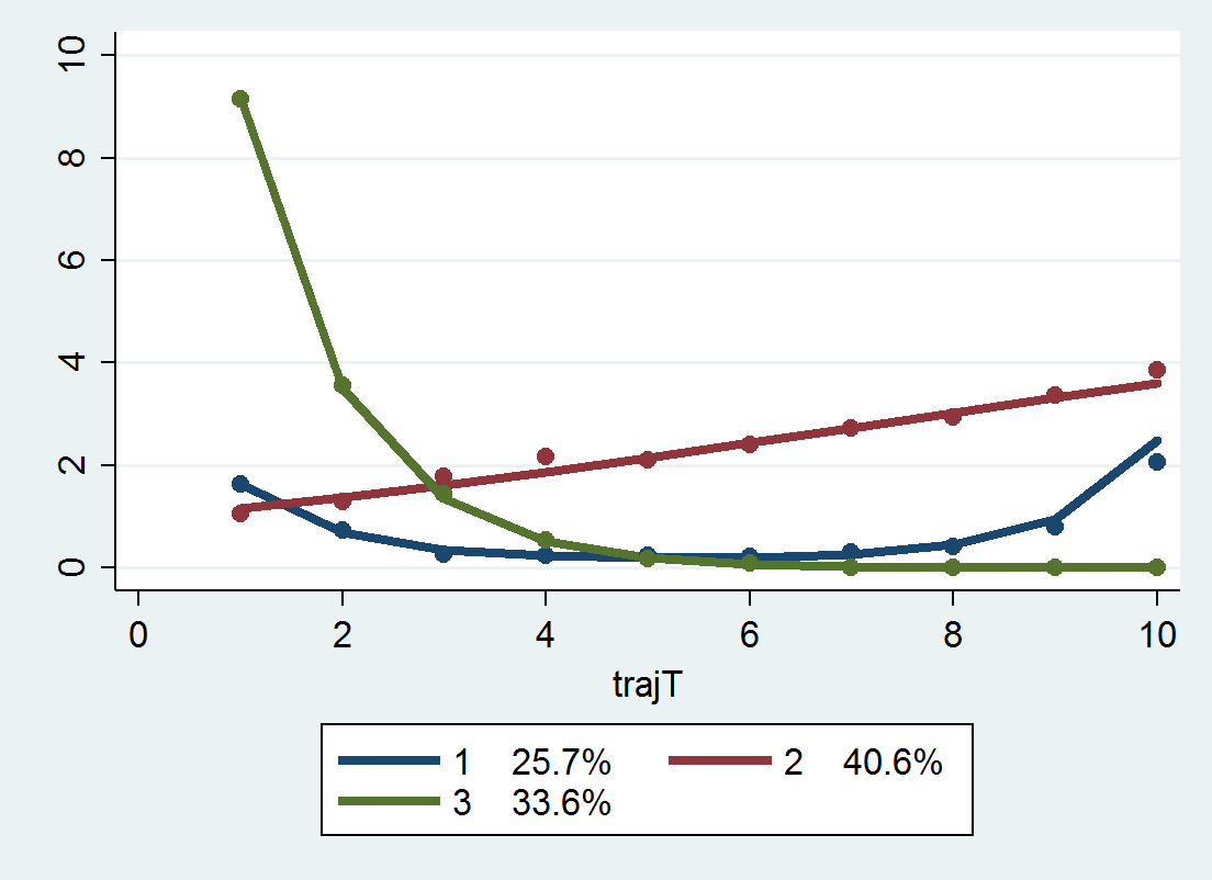

Now for absolute model fit statistics, there are the average posterior probabilities, the odds of correct classification, and the observed classification proportion versus the expected classification proportion. Here I made a program that I will surely be ashamed of later (I should not brutalize the data and do all the calculations in matrix), but it works and produces an ugly table to get us these stats.

*I made a function to print out summary stats
program summary_table_procTraj
    preserve
    *now lets look at the average posterior probability
	gen Mp = 0
	foreach i of varlist _traj_ProbG* {
	    replace Mp = `i' if `i' > Mp 
	}
    sort _traj_Group
    *and the odds of correct classification
    by _traj_Group: gen countG = _N
    by _traj_Group: egen groupAPP = mean(Mp)
    by _traj_Group: gen counter = _n
    gen n = groupAPP/(1 - groupAPP)
    gen p = countG/ _N
    gen d = p/(1-p)
    gen occ = n/d
    *Estimated proportion for each group
    scalar c = 0
    gen TotProb = 0
    foreach i of varlist _traj_ProbG* {
       scalar c = c + 1
       quietly summarize `i'
       replace TotProb = r(sum)/ _N if _traj_Group == c 
    }
	gen d_pp = TotProb/(1 - TotProb)
	gen occ_pp = n/d_pp
    *This displays the group number [_traj_~p], 
    *the count per group (based on the max post prob), [countG]
    *the average posterior probability for each group, [groupAPP]
    *the odds of correct classification (based on the max post prob group assignment), [occ] 
    *the odds of correct classification (based on the weighted post. prob), [occ_pp]
    *and the observed probability of groups versus the probability [p]
    *based on the posterior probabilities [TotProb]
    list _traj_Group countG groupAPP occ occ_pp p TotProb if counter == 1
    restore
end

This should work after any model as long as the naming conventions for the assigned groups are _traj_Group and the posterior probabilities are in the variables _traj_ProbG*. So when you run

summary_table_procTraj

You get this ugly table:

     | _traj_~p   countG   groupAPP        occ     occ_pp       p    TotProb |
     |-----------------------------------------------------------------------|
  1. |        1      103   .9379318   43.57342   43.60432   .2575   .2573645 |
104. |        2      136   .9607258   47.48513   48.30997     .34   .3361462 |
240. |        3      161   .9935605   229.0413   225.2792   .4025   .4064893 |

The groupAPP are the average posterior probabilities – here you can see they are all quite high. occ is the odds of correct classification, and again they are all quite high. Update: Jeff Ward stated that I should be using the weighted posterior proportions for the OCC calculation, not the proportions based on the max. post. probability (that I should be using TotProb in the above table instead of p). So I have updated to include an additional column, occ_pp based on that suggestion. I will leave occ in though just to keep a paper trail of my mistake.

p is the proportion in each group based on the assignments for the maximum posterior probability, and the TotProb are the expected number based on the sums of the posterior probabilities. TotProb should be the same as in the Group Membership part at the bottom of the traj model. They are close (to 5 decimals), but not exactly the same (and I do not know why that is the case).

Next, to generate a plot of the individual trajectories, I want to reshape the data to long format. I use preserve in case I want to go back to wide format later and estimate more models. If you need to look to see how the reshape command works, type help reshape at the Stata prompt. (Ditto for help on all Stata commands.)

preserve
reshape long count_ t_, i(id)

To get the behavior I want in the plot, I use a scatter plot but have them connected via c(L). Then I create small multiples for each trajectory group using the by() option. Before that I slightly jitter the count data, so the lines are not always perfectly overlapped. I make the lines thin and grey — I would also use transparency but Stata graphs do not support this.

gen count_jit = count_ + ( 0.2*runiform()-0.1 )
graph twoway scatter count_jit t_, c(L) by(_traj_Group) msize(tiny) mcolor(gray) lwidth(vthin) lcolor(gray)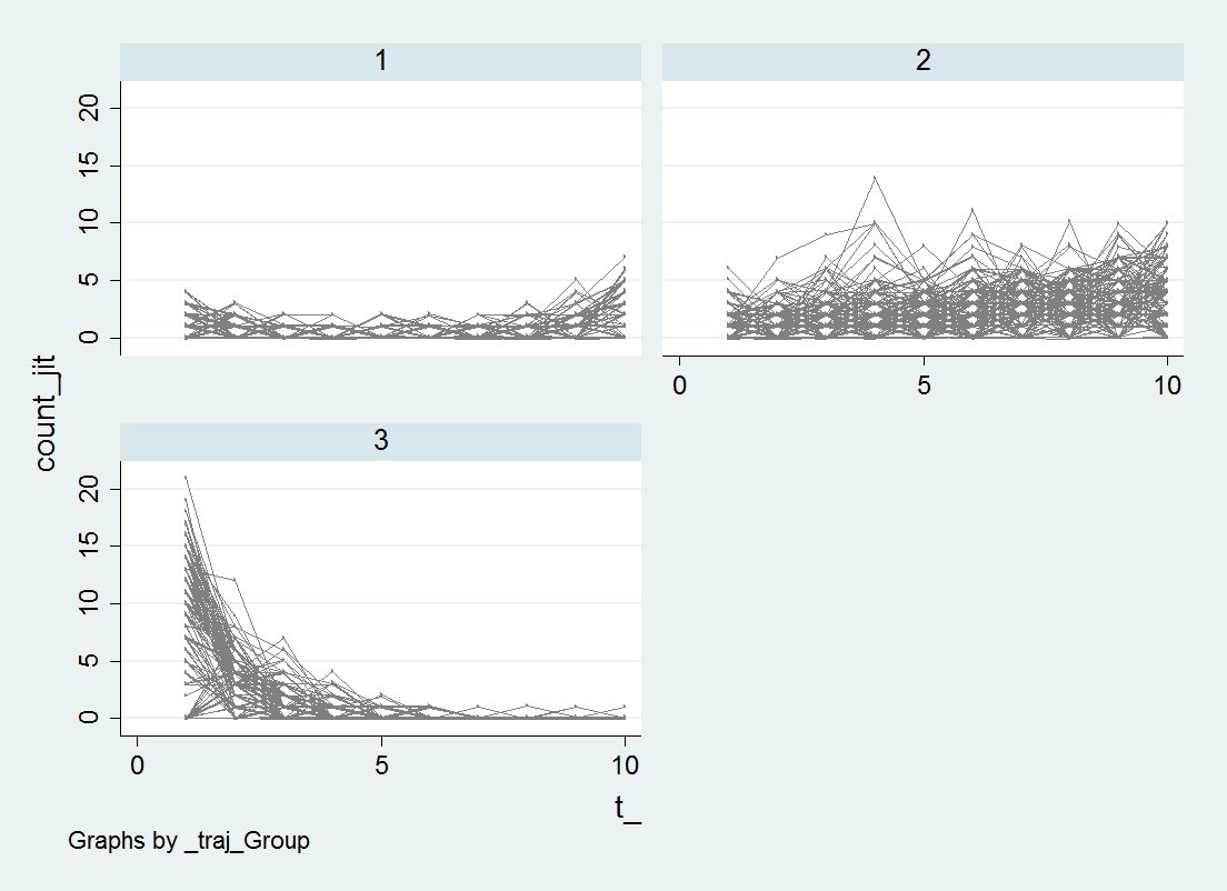

I’m too lazy at the moment to clean up the axis titles and such, but I think this plot of the individual trajectories should always be done. See Breaking Bad: Two Decades of Life-Course Data Analysis in Criminology, Developmental Psychology, and Beyond (Erosheva et al., 2014).

While this fit looks good, this is not the correct number of groups given how I simulated the data. I will give those trying to find the right answer a few hints; none of the groups have a higher polynomial than 2, and there is a constant zero inflation for the entire sample, so iorder(0) will be the correct specification for the zero inflation part. If you take a stab at it let me know, I will fill you in on how I generated the simulation.