A variance-covariance matrix expresses linear relationships between variables. Given the covariances between variables, did you know that you can write down an invertible linear transformation that "uncorrelates" the variables? Conversely, you can transform a set of uncorrelated variables into variables with given covariances. The transformation that works this magic is called the Cholesky transformation; it is represented by a matrix that is the "square root" of the covariance matrix.

The Square Root Matrix

Given a covariance matrix, Σ, it can be factored uniquely into a product Σ=UTU, where U is an upper triangular matrix with positive diagonal entries and the superscript denotes matrix transpose. The matrix U is the Cholesky (or "square root") matrix. Some people (including me) prefer to work with lower triangular matrices. If you define L=UT, then Σ=LLT. This is the form of the Cholesky decomposition that is given in Golub and Van Loan (1996, p. 143). Golub and Van Loan provide a proof of the Cholesky decomposition, as well as various ways to compute it.

Geometrically, the Cholesky matrix transforms uncorrelated variables into variables whose variances and covariances are given by Σ. In particular, if you generate p standard normal variates, the Cholesky transformation maps the variables into variables for the multivariate normal distribution with covariance matrix Σ and centered at the origin (denoted MVN(0, Σ)).

The Cholesky Transformation: The Simple Case

Let's see how the Cholesky transofrmation works in a very simple situation. Suppose that you want to generate multivariate normal data that are uncorrelated, but have non-unit variance. The covariance matrix for this situation is the diagonal matrix of variances: Σ = diag(σ21,...,σ2p). The square root of Σ is the diagonal matrix D that consists of the standard deviations: Σ = DTD where D = diag(σ1,...,σp).

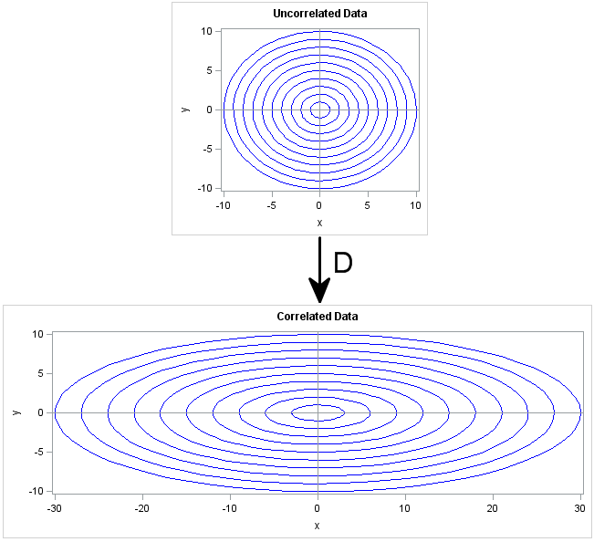
Geometrically, the D matrix scales each coordinate direction independently of the other directions. This is shown in the following image. The X axis is scaled by a factor of 3, whereas the Y axis is unchanged (scale factor of 1). The transformation D is diag(3,1), which corresponds to a covariance matrix of diag(9,1). If you think of the circles in the top image as being probability contours for the multivariate distribution MVN(0, I), then the bottom shows the corresponding probability ellipses for the distribution MVN(0, D).

The General Cholesky Transformation Correlates Variables

In the general case, a covariance matrix contains off-diagonal elements. The geometry of the Cholesky transformation is similar to the "pure scaling" case shown previously, but the transformation also rotates and shears the top image.

Computing a Cholesky matrix for a general covariance matrix is not as simple as for a diagonal covariance matrix. However, you can use ROOT function in SAS/IML software to compute the Cholesky matrix. Given any covariance matrix, the ROOT function returns a matrix U such that the product UTU equals the covariance matrix and U is an upper triangular matrix with positive diagonal entries. The following statements compute a Cholesky matrix in PROC IML:

proc iml;
Sigma = {9 1, 
         1 1};
U = root(Sigma);
print U (U`*U)[label="Sigma=U`*U"];

You can use the Cholesky matrix to create correlations among random variables. For example, suppose that X and Y are independent standard normal variables. The matrix U (or its transpose, L=UT) can be used to create new variables Z and W such that the covariance of Z and W equals Σ. The following SAS/IML statements generate X and Y as rows of the matrix xy. That is, each column is a point (x,y). (Usually the variables form the columns, but transposing xy makes the linear algebra easier.)The statements then map each (x,y) point to a new point, (z,w), and compute the sample covariance of the Z and W variables. As promised, the sample covariance is close to Σ, the covariance of the underlying population.

/* generate x,y ~ N(0,1), corr(x,y)=0 */
xy = j(2, 1000);
call randseed(12345);
call randgen(xy, "Normal"); /* each col is indep N(0,1) */
 
L = U`; 
zw = L * xy; /* apply Cholesky transformation to induce correlation */
cov = cov(zw`); /* check covariance of transformed variables */
print cov;

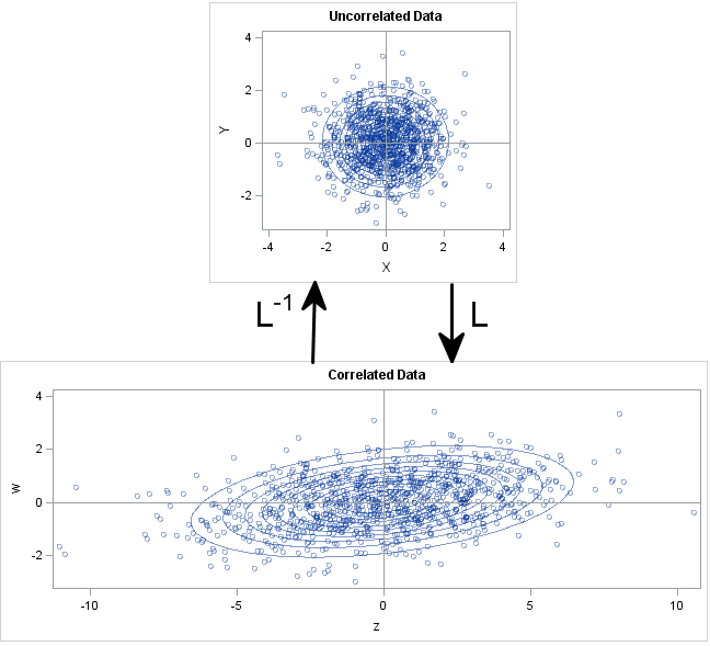
The following graph shows the geometry of the transformation in terms of the data and in terms of probability ellipses. The top graph is a scatter plot of the X and Y variables. Notice that they are uncorrelated and that the probability ellipses are circles. The bottom graph is a scatter plot of the Z and W variables. Notice that they are correlated and the probability contours are ellipses that are tilted with respect to the coordinate axes. The bottom graph is the transformation under L of points and circles in the top graph.

The Inverse Cholesky Transformation Uncorrelates Variables

You might wonder: Can you go the other way? That is, if you start with correlated variables, can you apply a linear transformation such that the transformed variables are uncorrelated? Yes, and it's easy to guess the transformation that works: it is the inverse of the Cholesky transformation!

Suppose that you generate multivariate normal data from MVN(0,Σ). You can "uncorrelate" the data by transforming the data according to L-1. In SAS/IML software, you might be tempted to use the INV function to compute an explicit matrix inverse, but as I have written, an alternative is to use the SOLVE function, which is more efficient than computing an explicit inverse matrix. However, since L is a lower triangular matrix, there is an even more efficient way to solve the linear system: use the TRISOLV function, as shown in the following statements:

/* Start with correlated data. Apply inverse of L. */
zw = T( RandNormal(1000, {0, 0}, Sigma) );
xy = trisolv(4, L, zw); /* more efficient than inv(L)*zw or solve(L, zw) */
 
/* did we succeed? Compute covariance of transformed data */
cov = cov(xy`);
print cov;

Success! The covariance matrix is essentially the identity matrix. The inverse Cholesky transformation "uncorrelates" the variables.

The TRISOLV function, which uses back-substitution to solve the linear system, is extremely fast. Anytime you are trying to solve a linear system that involves a covariance matrix, you should try to solve the system by computing the Cholesky factor of the covariance matrix, followed by back-substitution.

In summary, you can use the Cholesky factor of a covariance matrix in several ways:

• To generate multivariate normal data with a given covariance structure from uncorrelated normal variables.
• To remove the correlations between variables. This task requires using the inverse Cholesky transformation.
• To quickly solve linear systems that involve a covariance matrix.