Vector-based pedestrian navigation in cities

How do pedestrians choose their paths within city street networks? Researchers have tried to shed light on this matter through strictly controlled experiments, but an ultimate answer based on real-world mobility data is still lacking. Here, we analyze salient features of human path planning through a statistical analysis of a massive dataset of GPS traces, which reveals that (1) people increasingly deviate from the shortest path when the distance between origin and destination increases and (2) chosen paths are statistically different when origin and destination are swapped. We posit that direction to goal is a main driver of path planning and develop a vector-based navigation model; the resulting trajectories, which we have termed pointiest paths, are a statistically better predictor of human paths than a model based on minimizing distance with stochastic effects. Our findings generalize across two major US cities with different street networks, hinting to the fact that vector-based navigation might be a universal property of human path planning.

Although path planning is one of the hardest problems to solve computationally1, humans plan remarkably efficient paths when navigating cities, and do so at various scales. Although human path planning can be near-optimal, it also exhibits systematic divergences from the shortest available path2,3,4, and these divergences are still not well understood. We hypothesize that a contribution to such divergences arises from a common mental computational mechanism, which is shared among humans, that can be modeled in precise quantitative terms, and generalizes across urban environments. Describing this mechanism by a formal computational account can help explain mental computations in the brain that support human mobility, inform the design of real-time planning tools that can better couple human and machine intelligence, and improve urban planning.

In the laboratory setting, humans often rely on the ‘approximate rationality principle’, whereby humans use approximate planning heuristics to maximize their goals, while limiting subjective costs5,6,7,8,9. In the real world, these costs may be a combination of mental and physical effort10; for example, the mental cost of planning a route comes with the physical cost of travel. Multiple studies have investigated aggregate mobility flows11,12,13,14,15,16,17,18,19,20,21 and the cognitive abilities that support navigation22,23,24,25,26,27,28,29. Quantitative models of how humans may plan their routes in real cities have also been proposed, although these are limited to a small neighborhood in which the planning problem could be optimally solved with exhaustive route enumeration by a ‘breadth-first search’4. However, generalizable computational models that can generate precise quantitative predictions in large-scale city environments are still lacking. It is thus unclear which subjective costs and planning heuristics may explain human routes in real urban environments.

In this Article, we investigate this question by analyzing a large dataset of GPS traces of 552,478 pseudo-anonymized human paths undertaken by 14,380 pedestrians in two major US cities—Boston and San Francisco (Methods). The original dataset was retrieved from a company that runs one of the largest mobile apps for mobility tracking. With full consent from users, the app records high-resolution trajectories of human movements in complex urban environments while going about their daily life. Activity types have been labeled by the company using proprietary machine learning tools; only activities labeled as ‘walking path’ were analyzed in this work. Unlike previous studies of aggregate human mobility, which mostly rely on sparse location sampling (such as the serial numbers of US banknotes12, surveys18,30, commuting trips20, mobile communication records13, social-media check-ins31,32 or location history15,17), we study high-resolution routes of individual pedestrians, reconstructed from their GPS traces. Thanks to pseudo-anonymization, which assigned a unique anonymous ID to each individual in the dataset, we could also associate multiple trajectories to the same individual, allowing the study of individual-level properties of pedestrian routes (Supplementary Section 5). Importantly, the majority of human trajectories in our dataset were substantially different from routes suggested by Google Maps (Supplementary Tables 1–3 and Supplementary Fig. 3), indicating the minimal bias introduced by machine-generated trajectories on our data. This property, along with recordings of multiple trips by the same individual and between the same locations, enabled us to fit and evaluate alternate quantitative models of pedestrian navigation. In particular, we restricted our attention to simple geometric, computational models that can be used to at least partially explain human navigation ability.

Evaluating paths based on distance

As a first approximation, consider a simple way to formalize the cost of a path as equal to its distance:

Here, \({{{\mathcal{P}}}}\) denotes a path connecting the origin to the destination, which is composed of a list of street segments S1, S2, …, and li denotes the walking distance along segment Si. Although this simple model captures the motivation to reduce distance, which is central to human planning33,34, several studies show that humans often deviate from the shortest paths2,11,26,34,35.

Indeed, Fig. 1a shows that the human paths recorded in our dataset were consistently longer than the shortest-distance path computed using the standard Dijkstra algorithm36. The tendency to deviate from the shortest path increases with distance between the origin and destination (Fig. 1b), which could be due to the increasing complexity of evaluating relatively longer paths, in line with the approximate rationality principle. However, it is also interesting to observe that most of the relative deviation from the shortest path is achieved by paths of length around 1 km, and only a modest further increasing deviation is observed for longer paths.

Fig. 1: Differences between human paths and shortest paths.

a, Aggregated comparisons of the lengths of human and shortest paths (y axis) in Boston and San Francisco, as a function of the Euclidean distance between the origin (O) and destination (D) (x axis). b, Relative differences between human and shortest path lengths (y axis) as a function of the Euclidean distance between origin and destination (x axis). In the top plot, the bars denote the interquartile range, and the lines demonstrate the change of median % deviation values with increased origin–destination separation. The lower plot is a frequency histogram of sample distribution over origin–destination separations in log scale. c, Two examples of the difference between human paths (in red) and their corresponding shortest paths (in blue). Map data © OpenStreetMap contributors.

Source data

Full size image

Stochastic distance minimization

The increasing deviation from the shortest path observed in the data could arise from uncertainty about the lengths of street segments, which leads to an accumulation of errors over time. Formally, we can describe this process by an error term in the evaluation of street segment lengths:

where the new cost function c(li) is obtained by applying a log-normally distributed random noise to the original street segment length li. The use of a log-normal distribution to model uncertainty in street length estimation is motivated by the widely accepted Weber–Fechner law of just noticeable difference37, which states that humans perceive measurable quantities on a logarithmic scale. We will refer to equation (1) as the ‘stochastic distance minimization’ model. The number of street segments in the cost function (1) tends to increase with the Euclidean distance separating the origin and destination. Hence, the deviation from the shortest distance tends to accumulate with increased separation between origin and destination, as we observed.

Importantly, in the Methods we show that this model predicts path choices to be symmetrical—the available paths are ranked in the same order of preference regardless of travel direction, which may not be the case in human paths. Navigation asymmetry has been demonstrated in the laboratory38,39,40,41 and empirically noted—although never statistically tested—in pedestrian flows35 and driving routes34. A well-established theory of navigation by line of sight predicts asymmetric routes by suggesting that people travel along straight lines of sight in the desired direction and, when their view is obstructed, establish a new line of sight11. Empirical findings in neuroscience42,43 and psychology25,38 further suggest that neural and mental representations of space and direction could lead to asymmetry in two ways. Landmark-based navigation, extensively documented in humans22,23,25,29 and animals44, may lead to asymmetric paths that depend on the distribution of views in the environment. Furthermore, many animals, such as rodents45, bats46,47 and cats48, rely on direction42,43,45,49,50 for vector navigation50,51. Human subjects in laboratory studies likewise rely on direction for navigation, taking a route to the first destination that begins in the direction of subsequent destinations52, and rely on neural representations of both Euclidian distance and direction to destination42. Several small-scale studies have found that human routes exhibit systematic biases, such as bias toward paths that begin with a longer initial segment39,40,41, or a southern bias53, which may contribute to asymmetries. However, such biases have not yet been computationally modeled, nor quantitatively evaluated, in large-scale urban environments.

If present in human paths, asymmetric routes would falsify the stochastic distance minimization model as the only main contributor to pedestrian path formation. We tested for asymmetry as follows. First, we tested for asymmetric path choices within the same individual repeatedly visiting any given two locations in either order. If present, such individual-level asymmetries could arise from a cognitive cost heuristic used to evaluate trajectories, which depends on direction, or from stochasticity in distance evaluation, followed by memorizing the planned routes. Second, to disambiguate these two scenarios, we tested for asymmetries in repeated paths aggregated over different pedestrians. Such an asymmetry would indicate a persistent quality of human path planning that cannot be explained by stochastic route learning, and thus may be attributed to a common direction-dependent cost heuristic. We performed extensive statistical asymmetry tests at both individual and aggregate levels (see Methods for details). The results of the tests, reported in Fig. 2, show a statistically significant asymmetry in individual walking trajectories, as well as in aggregate trajectories, suggesting that asymmetries are a persistent quality of pedestrian navigation in urban street networks (see Methods for details).

Fig. 2: Asymmetric human paths.

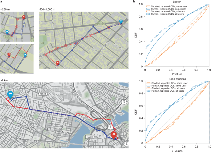
a, Examples of asymmetric human paths in street networks. Red paths start at red markers and blue paths at blue markers. b, Cumulative distribution function (CDF) of one-tailed P values for the asymmetry test in Boston and San Francisco (Methods). P values consistently above the diagonal dashed line indicate a statistically significant deviation from symmetric paths. Solid lines refer to individual-level tests and dotted lines to aggregate-level tests. Shortest-distance paths used in the tests are obtained by simulating the stochastic distance minimization model. Map data © OpenStreetMap contributors.

Source data

Full size image

Vector-based navigation model

Other geometric models, such as the ‘initial straightest segment’ (ISS) strategy proposed by Bailenson et al. in ref. 40, could be used to explain the observed asymmetry in human paths. If humans manifested a preference for the straightest first segment, we would expect to observe relatively longer first road segments in the human path than in the shortest path. However, human paths have consistently shorter initial segments than shortest paths, hinting that the ISS strategy is probably not a cause of the observed asymmetry (Supplementary Section 5.2).

Inspired by the evidence of asymmetry in human paths and the prevalence of vector navigation in animal models, we then hypothesized that humans use direction when planning their paths. We formalize the ‘vector-based navigation model’ as a cost that depends on the angular deviation of the street segment from the destination:

where

and θi ∈ [−π, π] represents the angle between the tangent to the path at street segment Si and the straight line to the destination (Fig. 3). In the example reported in Fig. 3a, the stochastic distance minimization model using equation (1) slightly prefers the blue path (for which ∑li = 935 m) over the red path (∑li = 938 m). The vector-based navigation model prefers what we call the pointiest path, meaning the path that more directly points towards the destination, which in this case is the red path (∑∣θi∣li = 400 m rad) over the blue path (∑∣θi∣li = 516 m rad). Because the angular deviations of street segments in this model depend on direction, the cost estimate of a path may change if its direction is reversed, implying that vector-based navigation could explain the asymmetries observed in human trajectories (see Methods for a detailed proof).

Fig. 3: Model design.

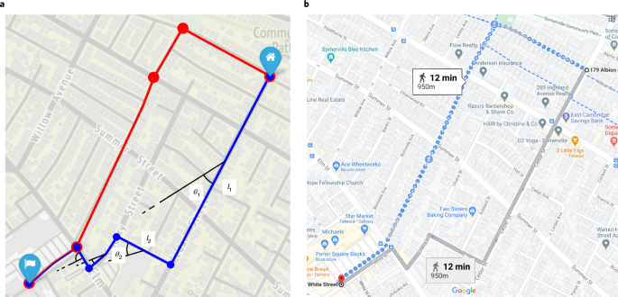
Example illustrating the calculation of the vector-based cost approximated by equation (2). a, The human path is shown in red and the shortest path in blue. The quantities li and θi appearing in equations (1) and (2) are shown for the first street segment of the blue path. b, Alternate paths produced by Google Maps. (Note that Google reports both path lengths as 950 m.) Map data © OpenStreetMap contributors.

Full size image

Model comparison

Having formally defined the two models, we compared their explanatory power relative to each other. We aggregated all paths by origin–destination (OD) distance separation, in steps of 50 m, and estimated the most likely parameters for the stochastic distance minimization and for the vector-based model in each bin (Methods). We measured the fraction of paths in each bin for which the vector-based model had a higher pointwise likelihood than the stochastic distance minimization model, and we called this the directional prevalence fraction (DPF). A value higher than 50% would imply a higher probability that a class of paths is explained through the vector-based model than the stochastic distance minimization model. The results reported in Fig. 4 show that, for each bin of OD distance separation with enough samples to reach statistical significance (Supplementary Section 3), the DPF is consistently above 50%, suggesting the higher explanatory power of the vector-based model. The decreasing trend of the DPF function as OD distance separation increases can be consistently observed both in Boston and in San Francisco. Moreover, the value of the DPF function is very similar across the entire range of OD distance separation, ranging from a peak of 68% at 150-m separation—which corresponds to 35% better predictive power of the vector-based model versus the stochastic shortest distance model—to 53% at 1-km separation. For the sake of completeness, note that the σ parameters for both models reach overall different values, 0.44 and 1.06 for the stochastic vector-based and shortest path models in Boston and 0.42 and 1.1 in San Francisco. More details on the calibration process and the detailed shape of the σ function are reported in Supplementary Figs. 4 and 5.

Fig. 4: DPF for different OD separations.

Top: marginal frequency distributions of paths in Boston and San Francisco. Bottom: similar DPF patterns in Boston and San Francisco. Error bars are obtained from the 95% Wilson-score interval61.

Source data

Full size image

The decreasing trend of the DPF function suggests a metacognitive mental computational mechanism that trades off mental and physical costs during navigation. As the length of the planned path increases, humans probably shift from the relatively easier direction optimization strategy towards optimizing the distance to save physical effort and travel time. This hypothesis is also supported by the observed deviation of human trajectories from shorter paths, which tends to level off for paths longer than 1 km (recall Fig. 1). Observing this trend in two cities with drastically different street network topologies suggests that this mental process generalizes across city environments.

The data-driven approach used in this Article illustrates how large-scale observations of behavior in natural settings can be used to derive quantitative models of complex cognitive and physical tasks, and complements studies of cognition in the laboratory by providing a unique insight into how the different cognitive faculties work together in real life. Despite all the challenges of an uncontrolled real city environment—as well as the lack of information about users and their activities that limits the range of applicability of our findings—we have discovered behavioral trends that generalize across cities, attesting to the potential of big data in the fields of psychology and cognitive science.

Our results suggest that vector navigation may be a common property of human route planning in cities and also establish direct connections between the study of human mobility, human cognitive psychology and neuroscience. Empirical support of the vector navigation model by real human behavior provides evidence in favor of theoretical claims that human minds and brains represent both Euclidean maps and graphs of street networks, as suggested in previous work54. The quantitative cost models described in this work suggest a possible computational mechanism by which route planning may be implemented in the brain. However, more work is needed to overcome the limitations of our study (lack of information about users and their activity) and understand, for instance, the effect of individual differences and the extent to which people pre-plan their routes, use hierarchical map representations, develop routing habits and diversify path alternates as a result of map learning.

The requirement to implement precise falsifiable models has limited our study to factors that could be measured objectively and exactly—such as direction and distance—as well as a number of simplifying assumptions. Although our models assume that pedestrians have accurate map knowledge, future work should consider how human path planning may depend on mental representations of the street networks, which may include larger streets and omit secondary ones55. Future work should also consider other factors that can influence navigation decisions, to the extent that these factors can be quantitatively tracked—such as day of the week, sunlight, weather, trees, attractions, presence of crowds, fatigue, time of the day, neighborhood safety and elevation gradient—as well as individual differences in responsiveness to these factors.

Our results extend our understanding of human route planning, and could have significant implications for those areas where route planning is a basic mechanism, such as transportation, cognitive maps and real-time planning algorithms. We expect our methodology to be of even greater use with increasingly accurate 5G and 6G tracking data. The latter should allow monitoring on which side of the street someone is walking, the time spent at intersections, forward-facing direction and speed, supporting a more detailed investigation of internal planning mechanisms. Future models should account for walking speed, tendency to change direction at a red light, as well as tendency to consistently orient toward specific visual landmarks. We hope that our findings will stimulate new research exploring these connections.

Dataset description and preparation

The full dataset comprises 579,231 pseudo-anonymized human paths produced by 14,380 pedestrians—5,590 in Boston and 8,790 in San Francisco—recorded by an always-on pedestrian tracking smartphone application over a time period of one year. As is customary in research based on datasets acquired through mobile applications, we do not have information about the demographics of the population of app users, which thus does not necessarily represent an unbiased sample of the population in Boston and San Francisco. The two cities differ in street network geometry (Supplementary Fig. 1). The San Francisco street network is designed as a grid, while the Boston street network is highly irregular, for historical reasons. The app was continuously recording individuals’ movements throughout the day. Accordingly, the dataset consists of raw high-quality GPS traces, which include a range of pedestrian activities. The analysis reported in this Article focuses on activities that have been labeled as ‘walking activity’ by the app using proprietary machine learning algorithms. Also, due to privacy limitations, we have no information about user profiles, such as whether they are resident in the city, their level of familiarity with the environment and so on. The average recording gap is 15 s, and the positioning accuracy is within 10 m. The GPS traces were segmented to individual paths based on tracking continuity, with a path considered to end at a destination if the walking activity was paused for longer than 5 min. To preserve privacy, the origin and destination of each trip were randomly relocated within a 100-m radius centered at the original location. To remove any possible bias resulting from this randomization procedure, we trimmed the beginning and end of each path within this range. All paths were map-matched to the Open Street Map network available at www.openstreetmap.org using a hidden Markov chain algorithm56. We also screened all map-matched paths using the Douglas–Peucker (DP) algorithm57 to exclude any detours that could be caused by GPS jitters that were not fully removed by the trimming.

We analyzed a subset of walking paths, selected from the full dataset, that met the following criteria: (1) no straight-line paths and (2) a path was not more than 80% longer than the shortest possible path connecting the origin and destination. The 80% cutoff was taken as the 95% quantile. The first criterion removed straightforward (from a navigational perspective) paths. The second criterion was implemented to exclude multi-purpose trips, sight-seeing and exercise. We also excluded paths with a shortest network distance smaller than 200 m. After this pre-processing, 165,645 trajectories by 4,879 pedestrians from Boston and 189,075 trajectories by 7,372 pedestrians from San Francisco remained in the analysis, comprising ~60% of paths from the original dataset.

The paths in Boston had a mean length of 856.0 m (s.d. = 843.6 m) and the paths in San Francisco had a mean length of 868.1 m (s.d. = 912.1 m). Detailed aggregate statistics of the human paths included in the study are reported in Supplementary Table 1.

Street networks

We retrieved the street network of the city of Boston and San Francisco and their surrounding areas from Open Street Map (Supplementary Fig. 1). All walkable street segments were included to form the walkable street network, which is used consistently for all the following calculations and analyses, including, but not limited to, map-matching of the human path, calculation of the shortest path, and random walk paths.

We simplified the retrieved street networks to speed up the calculation by cleaning up redundant nodes and edges around intersections. Specifically, we grouped adjacent intersections into one by applying a hierarchical clustering using the complete linkage and network distance among nodes. We selected 30 m as the threshold of the diameter of the clusters through repeated experiments. This simplification eliminated unnecessary details around intersections, while preserving network topology. The street networks of Boston and San Francisco used in our data analysis are illustrated in Supplementary Fig. 1.

Walking paths

The GPS trajectories of human paths were map-matched to the walking street network from Open Street Map (Supplementary Section 1.1) using a hidden Markov chain algorithm56. The algorithm was implemented using the map-matching application programming interface (API) of GraphHopper (https://graphhopper.com/api/1/docs/map-matching/). A small number of paths that were not successfully matched were eliminated from the dataset. The map-matched human paths were projected onto the simplified network utilizing the link table between nodes in the original network and the simplified network (Supplementary Section 1.1). The summary statistics of the shortest paths in both Boston and San Francisco are shown in Supplementary Table 1.

For each human path, the corresponding shortest-distance path was calculated based on the street network from Open Street Map (Supplementary Section 1.1) using the classic Dijkstra’s algorithm implemented in the Python package of igraph-python (http://igraph.org/python/). The map-matched shortest paths were projected onto the simplified network utilizing the link table between nodes in the original network and the simplified network. The summary statistics of the shortest paths in both Boston and San Francisco are shown in the Supplementary Table 1. The trip velocity distribution is reported in Supplementary Fig. 2.

The Google paths were retrieved from the Google Map Routing API and map-matched to the original street network using the identical hidden Markov model algorithm as applied to the human paths. Because of resource limitations, we randomly extracted a subset of paths for the comparison between human and Google paths in Boston and San Francisco, respectively. We retrieved Google paths for 9,254 OD pairs in Boston and 1,492 OD pairs in San Francisco. The comparison was restricted to the human paths for which we could obtain a corresponding Google path between the given origin and destination. If multiple human paths existed for one OD pair, all human paths were compared separately to the Google path, and average similarity performances were taken for the comparison. All retrieved Google trajectories were map-matched to the original street networks before being projected onto the simplified network.

To examine the probability of pedestrians following app-planned paths, we compared human paths to paths planned by the most widely used routing app—Google Map. The results show that Google paths are significantly different from human paths. First, the length distribution of Google paths is significantly different from that of human paths in both cities (Supplementary Fig. 3). Metrics comparing the geometries of Google paths with the geometries of human paths also demonstrate a significant difference in Jaccard similarity measured as exact overlaps, and in geometric similarity measured using Hausdorff distance (Supplementary Tables 2 and 3).

Detection of asymmetries

To test whether the sample probability distribution of paths chosen between any specific OD pair depends on the direction, we needed to aggregate trips across OD pairs. However, because the sample size obtained by considering the original OD pair was limited, we also considered intermediate points in a trajectory as possible OD pairs. To achieve a sufficiently large sample size, we considered only OD pairs within a Euclidean separation distance between 200 m and 250 m, with at least 50 recorded paths, including at least 20 paths in each direction, that do not lie on a straight line path. We define a straight-line path for an OD if there exists a path that simplifies to two points with the DP algorithm57, with a cutoff of 30 m. Note that this approach is conservative, because a symmetric model must necessarily be symmetric at all scales.

For the individual-level asymmetry test, this criterion is met by 235 OD pairs generated by 73 pedestrians in San Francisco and by 316 OD pairs generated by 101 pedestrians in Boston. For the aggregate asymmetry analysis, we also include any OD pairs that have a sufficient number of paths combined between different pedestrians, giving 2,865 and 3,000 OD pairs in San Francisco and Boston, respectively. Note that a single pedestrian path could be counted multiple times by considering different sub-parts of the original trajectory.

Aggregate-level analysis is done as follows. For a specific OD pair, we consider the universe of all paths followed by humans in each direction, and represent them as an unordered set of street intersection points. For each intersection point, we record the occurrence of out-bound \({\rm{O}}{\rm{D}}^{\to }=\{{n}_{1}^{\to },... \ ,{n}_{m}^{\to }\}\) and in-bound \({\rm{O}}{\rm{D}}^{\leftarrow }=\{{n}_{1}^{\leftarrow },... \ ,{n}_{m}^{\leftarrow }\}\) paths. Individual-level analysis is done as follows. We group all paths taken by an individual between a specific OD pair, \({\rm{OD}}=\{{{{{\mathcal{P}}}}}_{1},\ldots ,{{{{\mathcal{P}}}}}_{m}\}\), to determine the universe of observed paths in each direction. We count the number of occurrences of these paths in the forward and reverse directions, defined as \({\rm{O}}{\rm{D}}^{\to }=\{{n}_{1}^{\to },\ldots ,{n}_{m}^{\to }\}\) and \({\rm{O}}{\rm{D}}^{\leftarrow }=\{{n}_{1}^{\leftarrow },\ldots ,{n}_{m}^{\leftarrow }\}\), and establish an analogy with the process of extracting with replacement marbles from an urn containing m different types of marble—one for each possible path. More specifically, the urn contains \({n}_{i}^{\to }+{n}_{i}^{\leftarrow }\) marbles of type i, for each i. Given this analogy, the observed group of paths in one direction, say OD→, can be seen as an instance of a random extraction of \({q}^{\to }={\sum }_{i}{n}_{i}^{\to }\) marbles from the urn. If the paths were symmetric—null hypothesis—the extraction would obey a multinomial distribution. We can thus apply the standard statistical hypothesis test to the null hypothesis that the observations from sets OD→ and OD← follow such a distribution. The results of the test, reported in Fig. 2, show that the null hypothesis can be rejected with a 0.05 significance threshold for 32% and 24% of the OD pairs for Boston and San Francisco, respectively, and that the cumulative distribution of the resulting P values is considerably skewed towards lower values than those expected under the null hypothesis. We thus find a statistically significant asymmetry in individual human paths.

The proposed statistical test, which applies to both individual- and aggregate-level analyses, builds on the analogy with the process of independently extracting m marbles from an urn. If the null hypothesis that paths are symmetric is true, there exists a set of probabilities {p1,..., pm} with \(\mathop{\sum }\nolimits_{i = 1}^{m}{p}^{i}=1\) associated to each path that are direction-independent. In such a case, the best estimates for such probabilities can be obtained as

with \({q}^{\leftarrow }=\mathop{\sum }\nolimits_{i = 1}^{m}{n}_{i}^{\leftarrow }\) and \({q}^{\to }=\mathop{\sum }\nolimits_{i = 1}^{m}{n}_{i}^{\to }\).

To assess the validity of the null hypothesis, we test whether the sample occurrences OD→ and OD← are statistically compatible with the process of repeatedly and independently extracting q→ + q← elements from an urn with m marbles (with replacement). The resulting distribution is multinomial and defined by probabilities Pi. The exact P value for the test cannot be obtained analytically; however, the likelihood-ratio test58 provides an asymptotic distribution in the case the null hypothesis holds. Specifically, the maximum likelihood estimate is

and the alternate model is

Finally, according to Wilks’ theorem 58, the likelihood-ratio statistic should converge to a chi square with m − 1 degrees of freedom:

The results of the test are reported in the main text. Because the underlying distribution on which the statistical test is performed is unknown, we proceed with a more conservative test based on a null sampled distribution. This implies that the real null expectation should be slightly below the first bisector, as depicted by the shortest distance P-value distribution in Fig. 2b.

Asymmetry proofs

To prove that the stochastic distance minimization model cannot explain asymmetry, consider the (random) cost \({{{{\mathcal{C}}}}}_{\rm{dist}}({\rm{O}}{\rm{D}}^{\to })\) of a path between a certain OD pair, and the cost \({{\mathcal{C}}}_{\rm{dist}}({\rm{O}}{\rm{D}}^{\leftarrow })\) of the reverse path. Because both costs are obtained as the sum of independent random variables, and the random variables considered in the summation are the same (except for their order), both \({{\mathcal{C}}}_{\rm{dist}}({\rm{O}}{\rm{D}}^{\to })\) and \({{\mathcal{C}}}_{\rm{dist}}({\rm{O}}{{\rm{D}}}^{\leftarrow })\) have the same probability distribution, which contradicts our empirical observations of asymmetric human paths.

To prove that the vector-based navigation model can explain asymmetry, note that, for a given path between origin and destination, the costs of the path in the forward and reverse directions, Cdir(OD→) and Cdir(OD←), are obtained from the summation of different random variables, because the value \({\theta }_{i}^{\to }\) for street segment Si in the forward direction is different from that of \({\theta }_{i}^{\leftarrow }\) in the reverse direction (Fig. 3). Thus, the probability distribution of Cdir(OD→) is different from that of Cdir(OD←), which implies that the stochastic distance minimization model can support the hypothesis of asymmetric human navigation.

Model fitting and comparison

We compared the explanatory power of the two models by performing a set of 1,000 simulations in Boston and San Francisco to optimally tune the error parameter σ for both the stochastic distance minimization and the vector-based model (details about the exploration ranges for σ are provided in Supplementary Section 3). Given a human path OD(h)→ from origin to destination, we ran both models on that OD pair for 1,000 simulations, and recorded the number of times each of the two models selected exactly path OD(h)→. To determine which of the two models performed statistically better in this task, we compared their respective likelihood values. The likelihood of a model is obtained from

that is, the sum over all N paths of the logarithm of the probability

of selecting the human path OD(h)→ for OD pair ODi, computed using the cost function of the specific model x = {dist, dir} with the optimal value σx for model x of the error parameter.

We aggregated paths into bins by OD separation, in steps of 50 m. For each bin we calibrated σ and tested model performances with a leave-one-out cross-validation59. Accordingly, we found the value of σ that maximizes the likelihood of Ns − 1 paths associated with bin s, and measured the likelihood of the out-of-sample path. We repeated this procedure by leaving out another path until we covered the whole set of paths in each bin. We also included a cutoff parameter c to account for paths with zero sample probability, which would cause divergence of the likelihood metric. This parameter was set to c = 1/Ns = 0.001, which is the expected minimal detectable probability with Ns = 1,000 simulations. A detailed exploration of the dependency of c is reported in Supplementary Section 3. However, we did not observe a substantial change in our results with different values of c.

Due to privacy constraint policies and a signed data usage agreement, we are not allowed to share the full GPS tracks considered in this work. For this reason, we generated a small sample of 100 trajectories for Boston. We also make available the pre-processed pedestrian street networks for Boston and San Francisco. The sample dataset and street network data can be accessed at Zenodo60. Figures 1c, 2a and 3a used basemap from Open Street Map (https://www.openstreetmap.org) under an Open Database license (https://www.openstreetmap.org/copyright). Figure 3b uses Google Map data (2021) under fair-use guidelines (https://about.google/brand-resource-center/products-and-services/geo-guidelines/#general-guidelines-copyright-fair-use). Source data are provided with this paper.

The version of PedNav package used in this study and a guide to reproducing the results is available through GitHub under a GNU GPL-3.0 license (https://github.com/cbongiorno/pednav). The specific version of the package used to generate the results in the current study is available at Zenodo60. A pseudo-code description of the algorithms used for human navigation based on stochastic distance minimization and vector navigation is reported in Supplementary Section 4.

References

P.S. and C.R. thank the Amsterdam Institute for Advanced Metropolitan Solutions, Enel Foundation, DOVER and all of the members of the MIT Senseable City Laboratory Consortium for supporting this research. This material is based on work supported by the Center for Brains, Minds and Machines (CBMM), funded by NSF STC award no. CCF-1231216. C.B. and A.R. acknowledge support from the MISTI/MITOR fund. A.R. acknowledges support from Compagnia di San Paolo. This work was performed using HPC resources from the ‘Mésocentre’ computing center of CentraleSupélec and Ecole Normale Supérieure Paris-Saclay supported by CNRS and Région Île-de-France. Y.Z. acknowledges B. Huang and the Chinese University of Hong Kong for supporting his academic visit at the MIT Senseable City Laboratory.

Affiliations

1. Senseable City Lab, Massachusetts Institute of Technology, Cambridge, MA, USA

   Christian Bongiorno, Yulun Zhou, Paolo Santi & Carlo Ratti

2. Université Paris-Saclay, CentraleSupélec, Mathématiques et Informatique pour la Complexité et les Systèmes, Gif-sur-Yvette, France

   Christian Bongiorno

3. Department of Urban Planning and Design, Faculty of Architecture, The University of Hong Kong, Pokfulam, Hong Kong, China

   Yulun Zhou

4. Department of Brain and Cognitive Sciences, Massachusetts Institute of Technology, Cambridge, MA, USA

   Marta Kryven & Joshua Tenenbaum

5. Department of Physics, Massachusetts Institute of Technology, Cambridge, MA, USA

   David Theurel

6. Dipartimento di Elettronica e Telecomunicazioni, Politecnico di Torino, Torino, Italy

   Alessandro Rizzo

7. Office of Innovation, New York University Tandon School of Engineering, Six MetroTech Center, New York, NY, USA

   Alessandro Rizzo

8. Istituto di Informatica e Telematica del CNR, Pisa, Italy

   Paolo Santi

Contributions

A.R. and P.S. conceived and supervised the research. C.B. and Y.Z. led and performed the exploratory data analysis. C.B. designed the asymmetry testing procedure, the stochastic modeling, the validation method and performed the simulations. Y.Z. processed the data, conducted statistical analyses and drafted the manuscript. M.K. and D.T. carried out exploratory modeling converging on the presented model. M.K. drafted the introduction, content related to cognitive science and neuroscience, as well as cognitive science research and methodology. C.R. contributed to conceptualize and design the research. J.T. provided conceptualization and feedback. All authors contributed to writing and revising the manuscript.

Corresponding author

Correspondence to Paolo Santi.

Competing interests

The authors declare no competing interests.

Peer review information Nature Computational Science thanks Nora Newcombe, Steven Weisberg, Daniel Montello and Laura Alessandretti for their contribution to the peer review of this work. Handling editor: Fernando Chirigati, in collaboration with the Nature Computational Science team.

Publisher’s note Springer Nature remains neutral with regard to jurisdictional claims in published maps and institutional affiliations.

Reprints and Permissions

• A new computational model for human navigation

  • Laura Alessandretti

  Nature Computational Science (2021)