

Pytorch入门教程16-Pytorch中模型的定义和参数初始化
source link: https://mathpretty.com/12694.html
Go to the source link to view the article. You can view the picture content, updated content and better typesetting reading experience. If the link is broken, please click the button below to view the snapshot at that time.

Pytorch入门教程16-Pytorch中模型的定义和参数初始化
摘要这一篇详细介绍Pytorch中模型定义的几种方法. 同时, 也简单介绍参数的初始化.
这一篇文章会详细的介绍一下Pytorch中模型构建的方法(构建Block的方法), 注意包含下面的几种形式:
- 自定义一个Block, 直接继承nn.Module;
- 使用Sequential Block的方式进行定义;
- 自定义forward函数;
- 将上面的几种方法进行混合;
除了介绍模型构建的方法, 我们还会介绍对模型中的参数进行不同的操作.
- 参数的获取与操作;
- 参数的初始化操作;
- 参数绑定;
Pytorch模型构建方法
Custom Block
首先是最常用的一种方式, 我们可以通过直接继承nn.Module, 对其进行修改, 来完成我们需要的网络结构. 例如下面是一个全连接网络的实现, 我们只需要完成init的部分, 和forward的部分. 关于参数初始化, 反向传播会由Pytorch框架来完成.
- class MLP(nn.Module):
- # Declare a layer with model parameters. Here, we declare two fully
- # connected layers
- def __init__(self):
- # Call the constructor of the MLP parent class Block to perform the
- # necessary initialization. In this way, other function parameters can
- # also be specified when constructing an instance, such as the model
- # parameter, params, described in the following sections
- super().__init__()
- self.hidden = nn.Linear(20,256) # Hidden layer
- self.out = nn.Linear(256,10) # Output layer
- # Define the forward computation of the model, that is, how to return the
- # required model output based on the input `x`
- def forward(self, x):
- # Note here we use the funtional version of ReLU defined in the
- # nn.functional module.
- return self.out(F.relu(self.hidden(x)))
在自定义init的时候, 我们需要需要首先使用super().init()来调用父类的init方法.
Sequential Block
下面是构建序列结构的方式. 在Pytorch中有默认的构建序列的方式, 我们可以使用nn.Sequential, 如下所示:
- net = nn.Sequential(nn.Linear(20, 256), nn.ReLU(), nn.Linear(256, 10))
同样, 我们也是可以进行自定义. 需要注意的是我们没有直接使用一个list来进行存储, 而是使用Module中的_modules的有序字典类型来进行存储. 这样使用的一个好处是, 在模型参数初始化的时候, 会对_modules进行sub-block同样进行初始化.
- class MySequential(nn.Module):
- def __init__(self, *args):
- super().__init__()
- for block in args:
- # Here, block is an instance of a Module subclass. We save it in
- # the member variable _modules of the Module class, and its type
- # is OrderedDict
- self._modules[block] = block
- def forward(self, x):
- # OrderedDict guarantees that members will be traversed in the order
- # they were added
- for block in self._modules.values():
- x = block(x)
- return x
使用的方法还是和上面的nn.Sequential是一样的, 传入我们需要的Block即可.
- net = MySequential(nn.Linear(20, 256), nn.ReLU(), nn.Linear(256, 10))
Executing Code in the forward Method
上面我们都是直接使用Pytorch中现成的模块. 我们也可以在其中自定义一些操作. 例如可以有Python中的控制流 (control flow); 同时, 我们也可以进行自定义的运算. 例如下面的例子.
- 首先是rand_weight是不需要计算梯度的, 也就是requires_grad=False.
- 同时, 在forward部分, 会有一个while循环.
- class FixedHiddenMLP(nn.Module):
- def __init__(self):
- super().__init__()
- # Random weight parameters that will not compute gradients and
- # therefore keep constant during training
- self.rand_weight = torch.rand((20, 20), requires_grad=False)
- self.linear = nn.Linear(20, 20)
- def forward(self, x):
- x = self.linear(x)
- # Use the constant parameters created, as well as the relu and dot
- # functions
- x = F.relu(torch.mm(x, self.rand_weight) + 1)
- # Reuse the fully connected layer. This is equivalent to sharing
- # parameters with two fully connected layers
- x = self.linear(x)
- # Here in Control flow, we need to call asscalar to return the scalar
- # for comparison
- while x.norm().item() > 1:
- return x.sum()
Mixed Block
最后我们看一个比较综合的应用, 将上面的几种定义Block的方法都集中起来.
- 总的是通过nn.Sequential来进行连接的.
- 第一个部分, NestMLP也是包含两个部分.
- 接着是一个nn.Linear
- 最后是一个上面定义的, 自定义了forward函数的Block.
- class NestMLP(nn.Module):
- def __init__(self):
- super().__init__()
- self.net = nn.Sequential(nn.Linear(20, 64), nn.ReLU(),
- nn.Linear(64, 32), nn.ReLU())
- self.linear = nn.Linear(32, 16)
- def forward(self, x):
- return self.linear(self.net(x))
- chimera = nn.Sequential(NestMLP(), nn.Linear(16, 20), FixedHiddenMLP())
Pytorch中的自定义Layer
上面我们讲了在Pytorch中, 如何构建整个模型, 这里再着重介绍一下每一个Layer如何进行自定义.
Layer中不包含系数
首先, 我们可以定义一个不包含参数的Layer, 如下面的, 我们是数据的均值为0.
- class CenteredLayer(nn.Module):
- def __init__(self):
- super().__init__()
- def forward(self, x):
- return x - x.mean()
例如, 当我们的输入是(1,2,3,4,5), 此时均值是3的时候, 输出为(-2,-1,0,1,2). 如下面例子所示.
- layer = CenteredLayer()
- layer(torch.FloatTensor([1, 2, 3, 4, 5]))
- tensor([-2., -1., 0., 1., 2.])
我们可以将我们定义的这一层很容易的加到整个网络中去.
- net = nn.Sequential(nn.Linear(8, 128), CenteredLayer())
Layer中包含参数
上面我们看了简单的Layer是如何进行定义的. 现在我们看一下当一个Layer中包含参数, 在训练的时候, 我们需要更新这些参数. 这个时候应该如何进行定义. 下面的例子, 我们实现了一个简单的全连接层的效果.
- class MyLinear(nn.Module):
- def __init__(self, in_units, units):
- super().__init__()
- self.weight = nn.Parameter(torch.randn(in_units, units))
- self.bias = nn.Parameter(torch.randn(units,))
- def forward(self, x):
- return torch.matmul(x, self.weight.data) + self.bias.data
同样, 我们可以使用我们定义的网络层来组成一个模型.
- net = nn.Sequential(MyLinear(64, 8), nn.ReLU(), MyLinear(8, 1))
- net(torch.randn(2, 64))
Pytorch网络参数的相关控制
在这一部分, 我们主要从模型参数的三个主要部分来进行介绍:
- Accessing parameters for debugging, diagnostics, and visualizations. (查看网络的参数)
- Parameter initialization.
- Sharing parameters across different model components.
Parameter Access
简单参数的获取
现在假设我们使用nn.Sequential来构建网络, 如下所示, 我们构建一个简单的全连接网络.
- net = nn.Sequential(nn.Linear(4, 8), nn.ReLU(), nn.Linear(8, 1))
那么, 当我们通过Sequential来进行定义的时候, 我们可以通过index的方式获得每一层的参数. 下面我们来看一下最后一层的参数. 最后是通过有序字典(OrderedDict)进行返回.
- print(net[2].state_dict())
- OrderedDict([('weight', tensor([[-0.3289, -0.3328, -0.2062, 0.0865, 0.2737, 0.3170, 0.0943, -0.0462]])), ('bias', tensor([0.1746]))])
我们看到第二个是激活函数ReLU, 他是没有系数的, 我们也是同样可以看一下.
- print(net[1].state_dict())
- OrderedDict()
上面只是返回了字典类型, 为了做一些更有用的操作, 我们需要获得他的数字的值(numerical values). 我们通过下面的方式进行获得.
- print(net[2].bias)
- print(net[2].bias.data)
- tensor([0.1746], requires_grad=True)
- tensor([0.1746])
除了获得上面的data之外, 我们还是可以获得gradients, 并对其进行设置. 看下面一个简单的例子.
- net[2].weight.grad == None
所有系数一起操作
有的时候我们需要对所有的系数一起进行操作, 上面的方法就会显得比较麻烦. 那么我们总体看一下整个网络的OrderedDict是什么样子的. 可以看到第一层的key是'0.weight'和'0.bias'. 也就是每一层会在前面加上编号.
- net.state_dict()
- OrderedDict([('0.weight', tensor([[-0.4401, 0.1671, -0.2557, -0.2542],
- [ 0.0476, -0.3741, 0.2795, 0.2561],
- [-0.1753, -0.3761, 0.2565, 0.2287],
- [-0.1435, -0.4030, 0.1671, 0.2304],
- [ 0.1131, 0.4255, -0.1356, 0.4474],
- [ 0.3750, -0.0760, 0.1078, -0.1561],
- [-0.1217, -0.3878, -0.3331, 0.3495],
- [ 0.0281, -0.2158, 0.3175, -0.0070]])),
- ('0.bias', tensor([ 0.2330, 0.2435, -0.3555, -0.3084, 0.0134, -0.4436, -0.4233, 0.0456])),
- ('2.weight', tensor([[-0.3289, -0.3328, -0.2062, 0.0865, 0.2737, 0.3170, 0.0943, -0.0462]])),
- ('2.bias', tensor([0.1746]))])
那么, 此时我们要获取某一层的系数, 就可以先获取整个net的系数, 接着按照key来进行索引. 下面是获得第二层的weight的值, 可以看到和之前获取的是一样的.
- net.state_dict()['2.weight'].data
- tensor([[-0.3289, -0.3328, -0.2062, 0.0865, 0.2737, 0.3170, 0.0943, -0.0462]])
系数初始化(Parameter Initialization)
上面我们介绍了如何获取网络中的系数, 下面我们来看一下如何对其进行初始化的操作. 我们的框架会随机对系数进行初始化, 但是有的时候我们会希望指定方法来进行初始化.
Built-in Initialization
首先我们看一下使用内置的初始话的方法. 也就是修改init的时候系数初始化的方法. 下面我们初始化的方法是:
- 将weight的系数初始化为, 均值=0, 方差=0.01的高斯分布;
- 将bias初始化为0;
- def init_normal(m):
- if type(m) == nn.Linear:
- nn.init.normal_(m.weight, mean=0, std=0.01)
- nn.init.zeros_(m.bias)
- net = nn.Sequential(nn.Linear(4, 8), nn.ReLU(), nn.Linear(8, 1))
- # 对net使用这个初始化的规则
- net.apply(init_normal)
- # 查看系数
- net[0].weight.data[0], net[0].bias.data[0]
- (tensor([ 0.0007, -0.0123, -0.0065, 0.0029]), tensor(0.))
除了上面的初始化的方法之外, 我们还可以将所有的系数都初始化为常数, 下面我们将所有的weight都设置为1, 所有的bias都设置为0:
- def init_constant(m):
- if type(m) == nn.Linear:
- nn.init.constant_(m.weight, 1)
- nn.init.zeros_(m.bias)
- net = nn.Sequential(nn.Linear(4, 8), nn.ReLU(), nn.Linear(8, 1))
- net.apply(init_constant)
- net[0].weight.data[0], net[0].bias.data[0]
- (tensor([1., 1., 1., 1.]), tensor(0.))
除此之外, 我们还可以对不同的layer进行不同的初始化操作, 如下所示:
- def xavier(m):
- if type(m) == nn.Linear:
- torch.nn.init.xavier_uniform_(m.weight)
- def init_42(m):
- if type(m) == nn.Linear:
- torch.nn.init.constant_(m.weight, 42)
- net[0].apply(xavier) # 使用Xavier initializer
- net[2].apply(init_42) # 初始化为常数
- print(net[0].weight.data[0])
- tensor([ 0.0454, -0.1850, 0.4538, 0.4998])
- print(net[2].weight.data)
- tensor([[42., 42., 42., 42., 42., 42., 42., 42.]])
Custom Initialization
有的时候, 有一些初始化的方法是框架没有提供的, 这个时候我们就需要进行自定义操作了. 上面用的初始化的方法, 比如初始化为全0, 全1或是高斯分布, 都是Pytorch中框架自带的. 我们只是对不同的层使用不同的初始化的方法.
但是现在我们要自己定义一个初始化的分布. 例如我们定义一个一下的分布, 用来初始化系数.
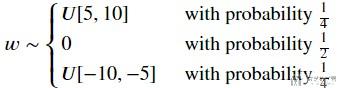
上面可以使用torch.nn.init来进行初始化, 这里我们就需要自行对系数进行操作. 例如下面, 当我们对weight进行初始化之后, 我们需要将[-5,5]之间都设置为0.
- def my_init(m):
- if type(m) == nn.Linear:
- nn.init.uniform_(m.weight, -10, 10)
- # print(m.weight)
- m.weight.data *= m.weight.data.abs() >= 5 # 只保留大于5或者小于-5的系数
- # print(m.weight)
- # 在[-10,10]之间的系数
- ensor([[-1.5157, 5.7350, 3.4442, -3.4822],
- [-4.8276, -4.6641, 3.5532, -9.3350],
- [ 8.3723, 3.6050, 7.3844, -9.5979],
- [-0.7135, 9.4364, 0.9190, 9.9970],
- [-8.1832, -8.9159, 8.3061, 8.8829],
- [ 4.4121, 2.8894, 6.2797, -7.7932],
- [-8.5017, -6.3802, 3.9993, -1.8441],
- [-6.8312, 9.8856, 9.0257, -5.2401]], requires_grad=True)
- # 只取得>5或是<-5
- tensor([[-0.0000, 5.7350, 0.0000, -0.0000],
- [-0.0000, -0.0000, 0.0000, -9.3350],
- [ 8.3723, 0.0000, 7.3844, -9.5979],
- [-0.0000, 9.4364, 0.0000, 9.9970],
- [-8.1832, -8.9159, 8.3061, 8.8829],
- [ 0.0000, 0.0000, 6.2797, -7.7932],
- [-8.5017, -6.3802, 0.0000, -0.0000],
- [-6.8312, 9.8856, 9.0257, -5.2401]], requires_grad=True)
同样, 我们还是使用apply来对目标网络的参数进行初始化.
- net.apply(my_init)
同时, 我们也是可以直接对系数进行修改的.
- net[0].weight.data[:] += 1
- net[0].weight.data[0, 0] = 42
- net[0].weight.data[0]
有的时候, 我们希望不同layer之间是可以共享系数的, 一个简单的方法就是首先在外面定义一层, 接着里面使用同一个block. 下面看一个简单的例子.
- shared = nn.Linear(8, 8)
- net = nn.Sequential(nn.Linear(4, 8), nn.ReLU(),
- shared, nn.ReLU(),
- shared, nn.ReLU(),
- nn.Linear(8, 1))
我们首先定义一个shared层, 接着在net的时候, 其中net[2]和net[4]都是使用的shared. 我们修改其中的一个系数.
- net[2].weight.data[0, 0] = 100
另外一个layer的系数也是会一起进行改变的.
- print(net[2].weight.data[0,0], net[4].weight.data[0,0])
- tensor(100.) tensor(100.)
那么此时这两层的系数是一样的, 我们如何进行反向传播呢. 在实际计算梯度的时候, 会对这两层的梯度值进行累加, 接着一起进行反向传播. (the gradients of the second hidden layer and the third hidden layer are added together during backpropagation.)
- 微信公众号
- 关注微信公众号
-

- QQ群
- 我们的QQ群号
-

Recommend
About Joyk
Aggregate valuable and interesting links.
Joyk means Joy of geeK