A Neighborhood of Infinity

Some pointers to things not in this blog

One reason I haven't blogged much recently is that my tolerance for blogger.com has reached its limit and I've been too lazy to build my own platform supporting mathematics and code. (For example, I can't get previewing on blogger to work today so I'm just publishing this and hope the reformatting is acceptable.) But that doesn't mean I haven't posted stuff publicly. So here are some thematically related links to things I've written on github and colab.

Read more »

Why does water fall out of an inverted cup?

Nuclear fusion

Is there any hope for fusion?

Preface

Functional programming encourages us to program without mutable state. Instead we compose functions that can be viewed as state transformers. It's a change of perspective that can have a big impact on how we reason about our code. But it's also a change of perspective that can be useful in mathematics and I'd like to give an example: a really beautiful technique that alows you to sample from the infinite limit of a probability distribution without needing an infinite number of operations. (Unless you're infinitely unlucky!)

Markov Chains

A Markov chain is a sequence of random states where each state is drawn from a random distribution that possibly depends on the previous state, but not on any earlier state. So it is a sequence such that for all . A basic example might be a model of the weather in which each day is either sunny or rainy but where it's more likely to be rainy (or sunny) if the previous day was rainy (or sunny). (And to be technically correct: having information about two days or earlier doesn't help us if we know yesterday's weather.)

Like imperative code, this description is stateful. The state at step depends on the state at step . Probability is often easier to reason about when we work with independent identically drawn random variables and our aren't of this type. But we can eliminate the state from our description using the same method used by functional programmers.

Let's choose a Markov chain to play with. I'll pick one with 3 states called , and and with transition probabilities given by where

Here's a diagram illustrating our states:

Implementation

First some imports:

> {-# LANGUAGE LambdaCase #-}
> {-# LANGUAGE TypeApplications #-}

> import Data.Sequence(replicateA) > import System.Random > import Control.Monad.State > import Control.Monad > import Data.List > import Data.Array

And now the type of our random variable:

> data ABC = A | B | C deriving (Eq, Show, Ord, Enum, Bounded)

We are now in a position to simulate our Markov chain. First we need some random numbers drawn uniformly from [0, 1]:

> uniform :: (RandomGen gen, MonadState gen m) => m Double
> uniform = state random

And now the code to take a single step in the Markov chain:

> step :: (RandomGen gen, MonadState gen m) => ABC -> m ABC
> step A = do
>     a <- uniform
>     if a < 0.5
>         then return A
>         else return B
> step B = do
>     a <- uniform
>     if a < 1/3.0
>         then return A
>         else if a < 2/3.0
>             then return B
>             else return C
> step C = do
>     a <- uniform
>     if a < 0.5
>         then return B
>         else return C

Notice how the step function generates a new state at random in a way that depends on the previous state. The m ABC in the type signature makes it clear that we are generating random states at each step.

We can simulate the effect of taking steps with a function like this:

> steps :: (RandomGen gen, MonadState gen m) => Int -> ABC -> m ABC
> steps 0 i = return i
> steps n i = do
>     i <- steps (n-1) i
>     step i

We can run for 100 steps, starting with , with a line like so:

*Main> evalState (steps 3 A) gen
B

The starting state of our random number generator is given by gen.

Consider the distribution of states after taking steps. For Markov chains of this type, we know that as goes to infinity the distribution of the th state approaches a limiting "stationary" distribution. There are frequently times when we want to sample from this final distribution. For a Markov chain as simple as this example, you can solve exactly to find the limiting distribution. But for real world problems this can be intractable. Instead, a popular solution is to pick a large and hope it's large enough. As gets larger the distribution gets closer to the limiting distribution. And that's the problem I want to solve here - sampling from the limit. It turns out that by thinking about random functions instead of random states we can actually sample from the limiting distribution exactly.

Some random functions

Here is a new version of our random step function:

> step' :: (RandomGen gen, MonadState gen m) => m (ABC -> ABC)
> step' = do
>     a <- uniform
>     return $ \case
>         A -> if a < 0.5 then A else B
>         B -> if a < 1/3.0
>                 then A
>                 else if a < 2/3.0 then B else C
>         C -> if a < 0.5 then B else C

In many ways it's similar to the previous one. But there's one very big difference: the type signature m (ABC -> ABC) tells us that it's returning a random function, not a random state. We can simulate the result of taking 10 steps, say, by drawing 10 random functions, composing them, and applying the result to our initial state:

> steps' :: (RandomGen gen, MonadState gen m) => Int -> m (ABC -> ABC)
> steps' n = do
>   fs <- replicateA n step'
>   return $ foldr (flip (.)) id fs

Notice the use of flip. We want to compose functions , each time composing on the left by the new . This means that for a fixed seed gen, each time you increase by 1 you get the next step in a single simulation: (BTW I used replicateA instead of replicateM to indicate that these are independent random draws. It may be well known that you can use Applicative instead of Monad to indicate independence but I haven't seen it written down.)

*Main> [f A | n <- [0..10], let f = evalState (steps' n) gen]
[A,A,A,B,C,B,A,B,A,B,C]

When I first implemented this I accidentally forgot the flip. So maybe you're wondering what effect removing the flip has? The effect is about as close to a miracle as I've seen in mathematics. It allows us to sample from the limiting distribution in a finite number of steps!

Here's the code:

> steps_from_past :: (RandomGen gen, MonadState gen m) => Int -> m (ABC -> ABC)
> steps_from_past n = do
>   fs <- replicateA n step'
>   return $ foldr (.) id fs

We end up building . This is still a composition of independent identically distributed functions and so it's still drawing from exactly the same distribution as steps'. Nonetheless, there is a difference: for a particular choice of seed, steps_from_past n no longer gives us a sequence of states from a Markov chain. Running with argument draws a random composition of functions. But if you increase by 1 you don't add a new step at the end. Instead you effectively restart the Markov chain with a new first step generated by a new random seed.

Try it and see:

*Main> [f A | n <- [0..10], let f = evalState (steps_from_past n) gen]
[A, A, A, A, A, A, A, A, A, A]

Maybe that's surprising. It seems to get stuck in one state. In fact, we can try applying the resulting function to all three states.

*Main> [fmap f [A, B, C] | n <- [0..10], let f = evalState (steps_from_past n) gen]
[[A,B,C],[A,A,B],[A,A,A],[A,A,A],[A,A,A],[A,A,A],[A,A,A],[A,A,A],[A,A,A],[A,A,A],[A,A,A]]

In other words, for large enough we get the constant function.

Think of it this way: If f isn't injective then it's possible that two states get collapsed to the same state. If you keep picking random f's it's inevitable that you will eventually collapse down to the point where all arguments get mapped to the same state. Once this happens, we'll get the same result no matter how large we take . If we can detect this then we've found the limit of as goes to infinity. But because we know composing forwards and composing backwards lead to draws from the same distribution, the limiting backward composition must actually be a draw from the same distribution as the limiting forward composition. That flip can't change what probability distribution we're drawing from - just the dependence on the seed. So the value the constant function takes is actually a draw from the limiting stationary distribution.

We can code this up:

> all_equal :: (Eq a) => [a] -> Bool
> all_equal [] = True
> all_equal [_] = True
> all_equal (a : as) = all (== a) as

> test_constant :: (Bounded a, Enum a, Eq a) => (a -> a) -> Bool > test_constant f = > all_equal $ map f $ enumFromTo minBound maxBound

This technique is called coupling from the past. It's "coupling" because we've arranged that different starting points coalesce. And it's "from the past" because we're essentially asking answering the question of what the outcome of a simulation would be if we started infinitely far in the past.

> couple_from_past :: (RandomGen gen, MonadState gen m, Enum a, Bounded a, Eq a) =>
>                   m (a -> a) -> (a -> a) -> m (a -> a)
> couple_from_past step f = do
>     if test_constant f
>         then return f
>         else do
>             f' <- step
>             couple_from_past step (f . f')

We can now sample from the limiting distribution a million times, say:

*Main> let samples = map ($ A) $ evalState (replicateA 1000000 (couple_from_past step' id)) gen

We can now count how often A appears:

*Main> fromIntegral (length $ filter (== A) samples)/1000000
0.285748

That's a pretty good approximation to , the exact answer that can be found by finding the eigenvector of the transition matrix corresponding to an eigenvalue of 1.

> gen = mkStdGen 669

Notes

The technique of coupling from the past first appeared in a paper by Propp and Wilson. The paper Iterated Random Functions by Persi Diaconis gave me a lot of insight into it. Note that the code above is absolutely not how you'd implement this for real. I wrote the code that way so that I could switch algorithm with the simple removal of a flip. In fact, with some clever tricks you can make this method work with state spaces so large that you couldn't possibly hope to enumerate all starting states to detect if convergence has occurred. Or even with uncountably large state spaces. But I'll let you read the Propp-Wilson paper to find out how.

Introduction

I've been reading a little about concentration inequalities recently. I thought it would be nice to see if you can use the key idea, if not the actual theorems, to reduce the complexity of computing the probability distribution of the outcome of stochastic simulations. Examples might include random walks, or queues.

The key idea behind concentration inequalities is that very often most of the probability is owned by a small proportion of the possible outcomes. For example, if we toss a fair coin enough (say ) times we expect the number of heads to lie within of the mean about 99.99% of the time despite there being different total numbers possible. The probable outcomes tend to concentrate around the expectation. On the other hand, if we consider not the total number of heads, but the possible sequences of tosses, there are possibilities, all equally likely. In this case there is no concentration. So a key ingredient here is a reduction operation: in this case reducing a sequence of tosses to a count of the number that came up heads. This is something we can use in a computer program.

I (and many others) have written about the "vector space" monad that can be used to compute probability distributions of outcomes of simulations and I'll assume some familiarity with that. Essentially it is a "weighted list" monad which is similar to the list monad except that in addition to tracking all possible outcomes, it also propagates a probability along each path. Unfortunately it needs to follow through every possible path through a simulation. For example, in the case of simulating coin tosses it needs to track different possiblities, even though we're only interested in the possible sums. If, after each bind operation of the monad, we could collect together all paths that give the same total then we could make this code much more efficient. The catch is that to collect together elements of a type the elements need to be comparable, for example instances of Eq or Ord. This conflicts with the type of Monad which requires that we can use the >>= :: m a -> (a -> m b) -> m b and return :: a -> m a functions with any types a and b.

I'm going to deal with this by adapting a technique presented by Oleg Kiselyov for efficiently implementing the Set monad. Instead of Set I'm going to use the Map type to represent probability distributions. These will store maps saying, for each element of a type, what the probability of that element is. So part of my code is going to be a direct translation of that code to use the Map type instead of the Set type.

> {-# LANGUAGE GADTs, FlexibleInstances #-}
> {-# LANGUAGE ViewPatterns #-}

> module Main where

> import Control.Monad > import Control.Arrow > import qualified Data.Map as M > import qualified Data.List as L

The following code is very similar to Oleg's. But for first reading I should point out some differences that I want you to ignore. The type representing a probability distribution is P:

> data P p a where
>     POrd :: Ord a => p -> M.Map a p -> P p a
>     PAny :: p -> [(a, p)] -> P p a

But note how the constructors take two arguments - a number that is a probability, in addition to a weighted Map or list. For now pretend that first argument is zero and that the functions called trimXXX act similarly to the identity:

> instance (Ord p, Num p) => Functor (P p) where
>     fmap = liftM

> instance (Ord p, Num p) => Applicative (P p) where > pure = return > (<*>) = ap

> instance (Ord p, Num p) => Monad (P p) where > return x = PAny 0 [(x, 1)] > m >>= f = > let (e, pdf) = unP m > in trimAdd e $ collect $ map (f *** id) pdf

> returnP :: (Ord p, Num p, Ord a) => a -> P p a > returnP a = POrd 0 $ M.singleton a 1

> unP :: P p a -> (p, [(a, p)]) > unP (POrd e pdf) = (e, M.toList pdf) > unP (PAny e pdf) = (e, pdf)

> fromList :: (Num p, Ord a) => [(a, p)] -> M.Map a p > fromList = M.fromListWith (+)

> union :: (Num p, Ord a) => M.Map a p -> M.Map a p -> M.Map a p > union = M.unionWith (+)

> scaleList :: Num p => p -> [(a, p)] -> [(a, p)] > scaleList weight = map (id *** (weight *))

> scaleMap :: (Num p, Ord a) => p -> M.Map a p -> M.Map a p > scaleMap weight = fromList . scaleList weight . M.toList

This is a translation of Oleg's crucial function that allows us to take a weighted list of probability distributions and flatten them down to a single probability distribution:

> collect :: Num p => [(P p a, p)] -> P p a
> collect []  = PAny 0 []
> collect ((POrd e0 pdf0, weight) : rest) =
>     let wpdf0 = scaleMap weight pdf0
>     in case collect rest of
>       POrd e1 pdf1 -> POrd (weight*e0+e1) $ wpdf0 `union` pdf1
>       PAny e1 pdf1 -> POrd (weight*e0+e1) $ wpdf0 `union` fromList pdf1
> collect ((PAny e0 pdf0, weight) : rest) =
>     let wpdf0 = scaleList weight pdf0
>     in case collect rest of
>       POrd e1 pdf1 -> POrd (weight*e0+e1) $ fromList wpdf0 `union` pdf1
>       PAny e1 pdf1 -> PAny (weight*e0+e1) $ wpdf0 ++ pdf1

But now I really must explain what the first argument to POrd and PAny is and why I have all that "trimming".

Even though the collect function allows us to reduce the number of elements in our PDFs, we'd like to take advantage of concentration of probability to reduce the number even further. The trim function keeps only the top probabilities in a PDF, discarding the rest. To be honest, this is the only point worth taking away from what I've written here :-)

When we throw away elements of the PDF our probabilities no longer sum to 1. So I use the first argument of the constructors as a convenient place to store the amount of probability that I've thrown away. The trim function keeps the most likely outcomes and sums the probability of the remainder. I don't actually need to keep track of what has been discarded. In principle we could reconstruct this value by looking at how much the probabilities in our trimmed partial PDFs fall short of summing to 1. But confirming that our discarded probability and our partial PDF sums to 1 gives a nice safety check for our code and can give us some warning if numerical errors start creeping in. I'll call the total discarded probability the tail probability.

Here is the core function to keep the top values. In this case is given by a global constant called trimSize. (I'll talk about how to do this better later.)

> trimList :: (Ord p, Num p) => [(a, p)] -> (p, [(a, p)])
> trimList ps =
>     let (keep, discard) = L.splitAt trimSize (L.sortOn (negate . snd) ps)
>     in (sum (map snd discard), keep)

> trimAdd :: (Ord p, Num p) => p -> P p a -> P p a > trimAdd e' (POrd e pdf) = > let (f, trimmedPdf) = trimList (M.toList pdf) > in POrd (e'+e+f) (M.fromList trimmedPdf) > trimAdd e' (PAny e pdf) = > let (f, trimmedPdf) = trimList pdf > in PAny (e'+e+f) trimmedPdf

> runP :: (Num p, Ord a) => P p a -> (p, M.Map a p) > runP (POrd e pdf) = (e, pdf) > runP (PAny e pdf) = (e, fromList pdf)

And now some functions representing textbook probability distributions. First the uniform distribution on a finite set. Again this is very similar to Oleg's chooseOrd function apart from the fact that it assigns weights to each element:

> chooseP :: (Fractional p, Ord p, Ord a) =>
>            [a] -> P p a
> chooseP xs = let p = 1/fromIntegral (length xs)
>              in POrd 0 $ fromList $ map (flip (,) p) xs

And the Bernoulli distribution, i.e. tossing a Bool coin that comes up True with probability :

> bernoulliP :: (Fractional p, Ord p) =>
>               p -> P p Bool
> bernoulliP p = POrd 0 $ fromList $ [(False, 1-p), (True, p)]

Now we can try a random walk in one dimension. At each step we have a 50/50 chance of standing still or taking a step to the right:

> random_walk1 :: Int -> P Double Int
> random_walk1 0 = returnP 0
> random_walk1 n = do
>     a <- random_walk1 (n-1)
>     b <- chooseP [0, 1]
>     returnP $ a+b

Below in main we take 2048 steps but only track 512 probabilities. The tail probability in this case is about . So only tracking 1/4 of the outcomes has had almost no impact on the numbers. This also illustrates why it is good to track the tail probabilities rather than inferring them from the missing probabilities in the bulk of the PDF - they can be so small they vanish compared to floating poimnt errors. We can afford to track a lot fewer than 512 (out of 2049 possible) outcomes and still have a good representative PDF.

Now here's a two-dimensional random walk for 32 steps. The tail probability is about so we are getting a reasonably representative PDF. We have to run fewer steps than before, however, because the space of possible outcomes spans two dimensions, meaning that reduction doesn't help as much as it does in one dimension.

> random_walk2 :: Int -> (Int, Int) -> P Double (Int, Int)
> random_walk2 0 (x, y) = returnP (x, y)
> random_walk2 n (x, y) = do
>     (x',y') <- random_walk2 (n-1) (x, y)
>     dx <- chooseP [-1, 1]
>     dy <- chooseP [-1, 1]
>     returnP (x'+dx, y'+dy)

One last simulation. This is a queing scenario. Tasks come in once every tick of the clock. There are four queues a task can be assigned to. A task is assigned to the shortest queue. Meanwhile each queue as a 1/4 probability of clearing one item at each tick of the clock. We build the PDF for the maximum length any queue has at any time.

The first argument to queue is the number of ticks of the clock. The second argument is the list of lengths of the queues. It returns a PDF, not just on the current queue size, but also on the longest queue it has seen.

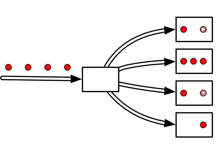
> queue :: Int -> [Int] -> P Double (Int, [Int])
> queue 0 ls = returnP (maximum ls, ls)
> queue n ls = do
>     (longest, ls1) <- queue (n-1) ls
>     ls2 <- forM ls1 $ \l -> do
>         served <- bernoulliP (1/4)
>         returnP $ if served && l > 0 then l-1 else l
>     let ls3 = L.sort $ head ls2+1 : tail ls2
>     returnP (longest `max` maximum ls3, ls3)

For the queing simulation the tail probability is around despite the fact that we have discarded a vast possible set of possible outcomes.

It's a little ugly that trimSize is a global constant:

> trimSize = 512

The correct solution is probably to separate the probability "syntax" from its "semantics". In other words, we should implement a free monad supporting the language of probability with suitable constructors for bernoulliP and choiceP. We can then write a separate interpreter which takes a trimSize as argument. This has another advantage too: the Monad above isn't a true monad. It uses a greedy approach to discarding probabilities and different rearrangements of the code, that ought to give identical results, may end up diferent. By using a free monad we ensure that our interface is a true monad and we can put the part of the code that breaks the monad laws into the interpreter. The catch is that my first attempt at writing a free monad resulted in code with poor performance. So I'll leave an efficient version as an exercise :-)

> main = do
>     print $ runP $ random_walk1 2048
>     print $ runP $ random_walk2 32 (0, 0)
>     print $ runP $ do
>         (r, _) <- queue 128 [0, 0, 0, 0]
>         returnP r