

Plotting Parametric Equations with JavaScript
source link: https://www.codedrome.com/plotting-parametric-equations-with-javascript/
Go to the source link to view the article. You can view the picture content, updated content and better typesetting reading experience. If the link is broken, please click the button below to view the snapshot at that time.

Parametric equations are used to calculate values, for example two dimensional or three dimensional coordinates, using an independent variable called a parameter.
In this article I will write a class which plots parametric equations in 3D using WebGL and the three.js library, and demonstrate its use with a few examples.
Parametric Equations - an Overview
You may have plotted functions in the form
y = f(x)
For example if you plot
y = x2
For the values of x between -10 and 10 you will get
Parametric equations work differently in that the values are calculated using an independent variable known as a parameter which is usually denoted by the letter t.
The simplest example is probably the pair of parametric equations for plotting a circle
x = cos(t)
y = sin(t)
To plot a circle we would iterate the parameter t from 0° to 360°, calculating and plotting the x and y coordinate for each angle.
There are plently of interesting and useful parametric equations which are plotted in just two dimensions and therefore have just two equations, one for the x coordinates and one for the y coordinates. However, we can extend the principle into three dimensions by adding an equation for the y coordinate. The code for this article allows us to do just that, and I will demonstrate with a few examples.
The Project
This project consists of the following files.
- parametricequations.htm
- parametricequationsplotter.js
- parametricequations.js
- parametricequationspage.js
- projects.css
You can download the source code as a ZIP or from the Github repository using the links below. The ZIP file and GitHub repository also include three.js.
Source Code Links
The HTML
The HTML is very simple, and includes an empty div which we will use to plot our parametric equations, as well as the various JavaScript files.
parametricequations.htm
<!DOCTYPE html>
<html lang="en">
<head>
<title>CodeDrome - Parametric Equations</title>
<meta charset="utf-8" />
<link href="projects.css" rel="stylesheet" />
</head>
<body>
<div class="maindiv">
<div class="banner"></div>
<div class="linkpanel"><a href="https://www.codedrome.com" target="_blank">codedrome.com</a></div>
<div id="container" class="roundcorners" style="position:absolute; top:58px; left:8px; right:8px; bottom:8px;">
</div>
</div>
<script src="three.js"></script>
<script src="parametricequations.js"></script>
<script src="parametricequationsplotter.js"></script>
<script src="parametricequationspage.js"></script>
</body>
</html>
The ParametricEquationsPlotter Class
The ParametricEquationsPlotter creates a three.js environment, and provides a method to plot parametric equations.
parametricequationsplotter.js
class ParametricEquationsPlotter
{
constructor()
{
this._container = null,
this._renderer = null,
this._scene = null,
this._light = null,
this._camera = null,
this._group = null,
this._meshlinematerial = null
this._createMaterials();
this._createScene();
this._drawMesh();
this._renderer.render(this._scene, this._camera);
}
_createMaterials()
{
this._meshlinematerial = new THREE.LineBasicMaterial({ color: 0x000000, transparent: true, opacity: 0.1 });
}
_createScene()
{
this._container = document.getElementById("container");
this._renderer = new THREE.WebGLRenderer({ antialias: true });
this._renderer.setSize(container.offsetWidth, container.offsetHeight);
this._container.appendChild(this._renderer.domElement);
this._scene = new THREE.Scene();
this._scene.background = new THREE.Color(0xFFFFFF);
this._camera = new THREE.PerspectiveCamera(45, this._container.offsetWidth / this._container.offsetHeight, 0.1, 20);
this._camera.position.set(0, 0, 5);
this._light = new THREE.DirectionalLight(0xFFFFFF, 2.0);
this._light.position.set(-1, 1, 1);
this._scene.add(this._light);
this._group = new THREE.Object3D();
this._scene.add(this._group);
this._group.rotation.x = 0.25;
this._group.rotation.y = 0.25;
// this._group.rotation.z = -0.5;
}
_drawMesh()
{
let points = null;
let geometry = null;
let line = null;
for(let x = -1; x <= 1; x++)
{
for(let y = -1; y <= 1; y++)
{
for(let z = -1; z <= 1; z++)
{
points = [new THREE.Vector3(x, y, z), new THREE.Vector3(x, y, -z)];
geometry = new THREE.BufferGeometry().setFromPoints( points );
line = new THREE.Line( geometry, this._meshlinematerial );
this._group.add(line);
points = [new THREE.Vector3(x, y, z), new THREE.Vector3(x, -y, z)];
geometry = new THREE.BufferGeometry().setFromPoints( points );
line = new THREE.Line( geometry, this._meshlinematerial );
this._group.add(line);
points = [new THREE.Vector3(x, y, z), new THREE.Vector3(-x, y, z)];
geometry = new THREE.BufferGeometry().setFromPoints( points );
line = new THREE.Line( geometry, this._meshlinematerial );
this._group.add(line);
}
}
}
}
Plot(xEquation, yEquation, zEquation, tRange, tStep, colour)
{
let xPrev = null, yPrev = null, zPrev = null;
let x = null, y = null, z = null;
let points = null, geometry = null, line = null;
const plotlinematerial = new THREE.LineBasicMaterial({ color: colour });
for(let t = tRange.start; t <= tRange.end; t += tStep)
{
x = xEquation(t);
y = yEquation(t);
z = zEquation(t);
if(xPrev !== null)
{
points = [new THREE.Vector3(xPrev, yPrev, zPrev), new THREE.Vector3(x, y, z)];
geometry = new THREE.BufferGeometry().setFromPoints( points );
line = new THREE.Line( geometry, plotlinematerial );
this._group.add(line);
}
xPrev = x;
yPrev = y;
zPrev = z;
}
this._renderer.render(this._scene, this._camera);
}
}
I won't go into the details of the three.js environment here as that is not the purpose of this article, but basically we need to create a container and add a renderer, a scene, a camera and one or more lights. I have also created a group to which we will add the components of the plot so that they can be manipulated as a single entity, for example changing the rotation. I have changed the x and y rotations slightly, and you can also change the z rotation if you wish by uncommenting the last line of the _createScene function.
The _drawMesh function draws a 3D box of lines to make it a bit easier to see how the plots fit in to the coordinate system: note that the centre of the box is 0,0,0.
The Plot method is central to the class, and takes six arguments:
- Equations for the x, y and z axes
- The range of the t parameter, an object with start and end properties
- The step or interval of the t parameter iteration
- The plot colour
After creating a few variables and a const material of the specified colour we iterate the t parameter across the specified range, with the specified interval.
Within the loop we calculate the x, y and z values by calling the respective functions, and then plot the point in 3D space. This is actually done by drawing a line from the previous point (unless we are at the first point) which, if the tStep argument is sufficiently small, should give a satisfactory illusion of a continuous curve.
Some Sample Parametric Equations
This file consists of a const object containing a number of other objects whose properties are the arguments needed by the Plot method to draw various shapes using parametric equations.
In most cases the tRange needs to be particular values, 0° to 360° (or actually the equivalent in radians), but for the spiral and helix they can be varied.
The ranges were set after a bit of trial and error to give reasonably smooth results.
For 2 dimensional equations the zFunction simply returns 0, although you could return another value to move the plot forwards or backwards along the y axis.
There are no less than four Lissajous curves here: you might like to read more about them on Wikipedia.
parametricequations.js
const ParametricEquations =
{
circle:
{
xFunction: function (t) {return Math.cos(t)},
yFunction: function (t) {return Math.sin(t)},
zFunction: function (t) {return 0},
tRange: {start: 0, end: 2 * Math.PI},
tStep: Math.PI / 32,
colour: "#FF0000"
},
ellipse:
{
xFunction: function (t) {return 1.0 * Math.cos(t)},
yFunction: function (t) {return 0.75 * Math.sin(t)},
zFunction: function (t) {return 0},
tRange: {start: 0, end: 2 * Math.PI},
tStep: Math.PI / 32,
colour: "#00C000"
},
cardioid:
{
xFunction: function (t) { return Math.cos(t) * (1 + Math.cos(t)) },
yFunction: function (t) { return Math.sin(t) * (1 + Math.cos(t)) },
zFunction: function (t) {return 0},
tRange: {start: 0, end: 2 * Math.PI},
tStep: Math.PI / 32,
colour: "#800080"
},
spiral:
{
xFunction: function (t) { return Math.cos(t) * (0.05 * t) },
yFunction: function (t) { return Math.sin(t) * (0.025 * t) },
zFunction: function (t) {return 0},
tRange: {start: 0, end: 10 * Math.PI},
tStep: Math.PI / 32,
colour: "#008080"
},
rose:
{
xFunction: function (t) { return Math.cos(t) * (Math.sin(t * 6)) },
yFunction: function (t) { return Math.sin(t) * (Math.sin(t * 6)) },
zFunction: function (t) {return 0},
tRange: {start: 0, end: 2 * Math.PI},
tStep: Math.PI / 128,
colour: "#FF00FF"
},
Lissajous1:
{
xFunction: function (t)
{
const delta = Math.PI / 2;
const a = 1;
return Math.sin(a * t + delta)
},
yFunction: function (t)
{
const b = 2;
return Math.sin(b * t)
},
zFunction: function (t) { return 0 },
tRange: {start: 0, end: 2 * Math.PI},
tStep: Math.PI / 128,
colour: "#FF8000"
},
Lissajous2:
{
xFunction: function (t)
{
const delta = Math.PI / 2;
const a = 3;
return Math.sin(a * t + delta)
},
yFunction: function (t)
{
const b = 2;
return Math.sin(b * t)
},
zFunction: function (t) { return 0 },
tRange: {start: 0, end: 2 * Math.PI},
tStep: Math.PI / 128,
colour: "#FF8000"
},
Lissajous3:
{
xFunction: function (t)
{
const delta = Math.PI / 2;
const a = 3;
return Math.sin(a * t + delta)
},
yFunction: function (t)
{
const b = 4;
return Math.sin(b * t)
},
zFunction: function (t) { return 0 },
tRange: {start: 0, end: 2 * Math.PI},
tStep: Math.PI / 128,
colour: "#FF8000"
},
Lissajous4:
{
xFunction: function (t)
{
const delta = Math.PI / 4;
const a = 5;
return Math.sin(a * t + delta)
},
yFunction: function (t)
{
const b = 4;
return Math.sin(b * t)
},
zFunction: function (t) { return 0 },
tRange: {start: 0, end: 2 * Math.PI},
tStep: Math.PI / 128,
colour: "#FF8000"
},
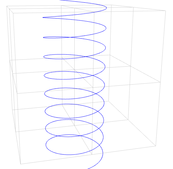
helix:
{
zFunction: function (t)
{
const a = 0.5; // radius
return a * Math.cos(t);
},
xFunction: function (t)
{
const a = 0.5; // radius
return a * Math.sin(t);
},
yFunction: function (t)
{
const b = 0.05; // height per revolution = 2pi * b
return b * t;
},
tRange: {start: -10 * Math.PI, end: 10 * Math.PI},
tStep: Math.PI / 128,
colour: "#0000FF"
},
}
Plotting the Equations
The final JavaScript file picks up one of the sets of values from the ParametricEquations object in parametricequations.js and calls the ParametricEquationsPlotter's Plot method.
parametricequationspage.js
"use strict"
window.onload = function()
{
const plotter = new ParametricEquationsPlotter();
const pe = ParametricEquations.circle;
// const pe = ParametricEquations.ellipse;
// const pe = ParametricEquations.cardioid;
// const pe = ParametricEquations.spiral;
// const pe = ParametricEquations.rose;
// const pe = ParametricEquations.Lissajous1;
// const pe = ParametricEquations.Lissajous2;
// const pe = ParametricEquations.Lissajous3;
// const pe = ParametricEquations.Lissajous4;
// const pe = ParametricEquations.helix;
plotter.Plot(pe.xFunction, pe.yFunction, pe.zFunction, pe.tRange, pe.tStep, pe.colour);
}
If you open the parametricequations.htm file in you browser you will get a circle, but you can uncomment the other lines one at a time to try out the other equations. (You can edit the code to plot more than one equation if you wish, but of course you'll need to give the consts different names.)
Here are a few examples, starting with a spiral. As I mentioned earlier, remember that the centre of the "box" is at 0,0,0.

...and a rose.

This is a Lissajous Curve...

... and finally a helix. If you feel like a bit of a challenge try plotting two helixes (or helices, both are correct!) to resemble a DNA double helix.
Other Equations
The field of parametric equations is vast and in this article I have only scratched the surface.
However, we now have a class which will plot any set of two or three parametric equations you might want to throw at it so experimenting with further equations is quite straightforward, or you might just want to try varying the arguments for the examples I have included.
If you want to discover more parametric equations take a look at the Wikipedia article. You might also like to look further into the fascinating topic of Lissajous curves.
Recommend
About Joyk
Aggregate valuable and interesting links.
Joyk means Joy of geeK