Helmhurts

A few posts back I was concerned with optimising the WiFi reception in my flat, and I chose a simple method for calculating the distribution of electromagnetic intensity. I casually mentioned that I really should be doing things more rigorously by solving the Helmholtz equation, but then didn’t. Well, spurred on by a shocking amount of spare time, I’ve given it a go here.

UPDATE: Android app now available, see this post for details.

The Helmholtz equation is used in the modelling of the propagation of electromagnetic waves. More precisely, if the time-dependence of an electromagnetic wave can be assumed to be of the form and the dispersion relation given by for some refractive index distribution , then the electric field solves

where is some source function. Given a source of radiation and a geometry to propagate in, in principle the Helmholtz equation can be solved for the entire radiation field . In practice this may not be so simple. Here I chose to model a situation in 2D, and set up a computational grid of size with grid cells labelled for , . Given this discretisation, the equation above becomes

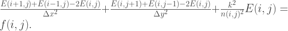
This is a linear equation in the ‘current’ cell as a function of its 4 neighbours. Each cell has an equation describing the relationship with its neighbours, so there are equations in unknowns. This motivates a linear algebraic approach to the problem – if all equations can be represented as one giant matrix equation, that matrix can be inverted and an exact solution for recovered. In particular we’ll have for some matrix , and we can compute .
This is slightly tricky due to the fact that a 2D labelling system needs to be converted to a 1D labelling system , as the 2D simulation domain needs to be converted to a 1D vector. I use the translation that so that

A pair of cells and are then separated by in this new labelling system, and a pair of cells and separated by 1.
The row in the matrix equation corresponding to the th cell looks like

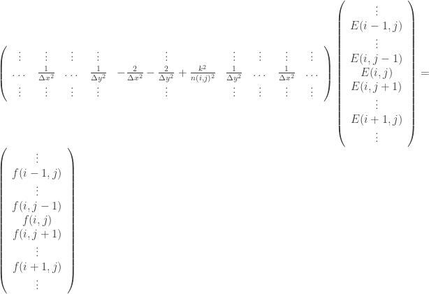
where there are blank cells between the and cells. In fact, it is clear that the vast majority of the matrix is zero, which can help when considering the sheer size of the matrix. For this problem a room is approximately 5 m across, and the wavelength to resolve is around 5 cm. We will require or so then, which means the number of elements is around ! Storing each as a single precision number would require around 60 GB of RAM, and my poor battered laptop wouldn’t have a chance inverting that matrix even if it would fit in memory.
Fortunately this problem has crept up on people cleverer than I, and they invented the concept of the sparse matrix, or a matrix filled mostly with zeros. We can visualise the structure of our matrix using the handy Matlab function spy – as plotted below it shows which elements of the matrix are nonzero.

Here , so there are 784 elements in the matrix. However only 64 of those are nonzero, just 8% of the matrix is actually useful in computation! This drops to 4% if the resolution of our grid jumps by a factor of 10, and stays around 5% for another factor of 10. There is a special data structure in Matlab for sparse matricies, and using it speeds up calculation of inverses by orders of magnitude. In this case the code is literally a hundred times faster and uses a fraction of the memory.
Moving on to the physics then, what does a solution of the Helmholtz equation look like? On the unit square for large , the quickest way is actually to use a packet of rice – see e.g. here.
In this calculation I’ve set boundary conditions that on the edges of the square, and set . It turns out that the Helmholtz equation can also be applied to the modelling of the forced vibrations of the square plate, where the choice of conditions above equates to applying a force at the centre of the plate and clamping the edges. The rice/sand/etc settles at the nodes of the plate, i.e. the positions which stay stationary in the oscillation.
Visualised below are a selected few pretty pictures where I’ve taken a logarithmic colour scale to highlight the positions of zero electric field – the ‘nodes’. As the animation proceeds starts high and gradually gets lower, corresponding to fast plate oscillations gradually getting slower.

Once again physics has turned out unexpectedly pretty and distracted me away from my goal, and this post becomes a microcosm of the entire concept of the blog…
Moving onwards, I’ll recap the layout of the flat where I’m hoping to improve the signal reaching my computer from my WiFi router:

I can use this image to act as a refractive index map – walls are very high refractive index, and empty space has a refractive index of 1. I then set up the WiFi antenna as a small radiation source hidden away somewhat uselessly in the corner. Starting with a radiation wavelength of 10 cm, I end up with an electromagnetic intensity map which looks like this:

This is, well, surprisingly great to look at, but is very much unexpected. I would have expected to see some region of ‘brightness’ around the electromagnetic source, fading away into the distance perhaps with some funky diffraction effects going on. Instead we get a wispy structure with filaments of strong field strength snaking their way around. There are noticeable black spots too, recognisable to anyone who’s shifted position in a chair and having their phone conversation dropped.

What if we stuck the router in the kitchen?

This seems to help the reception in all of the flat except the bedrooms, though we would have to deal with lightning striking the cupboard under the stairs it seems.

What about smack bang in the middle of the flat?

Thats more like it! Tendrils of internet goodness can get everywhere, even into the bathroom where no one at all occasionally reads BBC News with numb legs. Unfortunately this is probably not a viable option.

Actually the distribution of field strength seems extremely sensitive to every parameter, be it the position of the router, the wavelength of the radiation, or the refractive index of the front door. This probably requires some averaging over parameters or grid convergence scan, but given it takes this laptop 10 minutes or so to conjure up each of the above images, that’s probably out of the question for now.

UPDATE

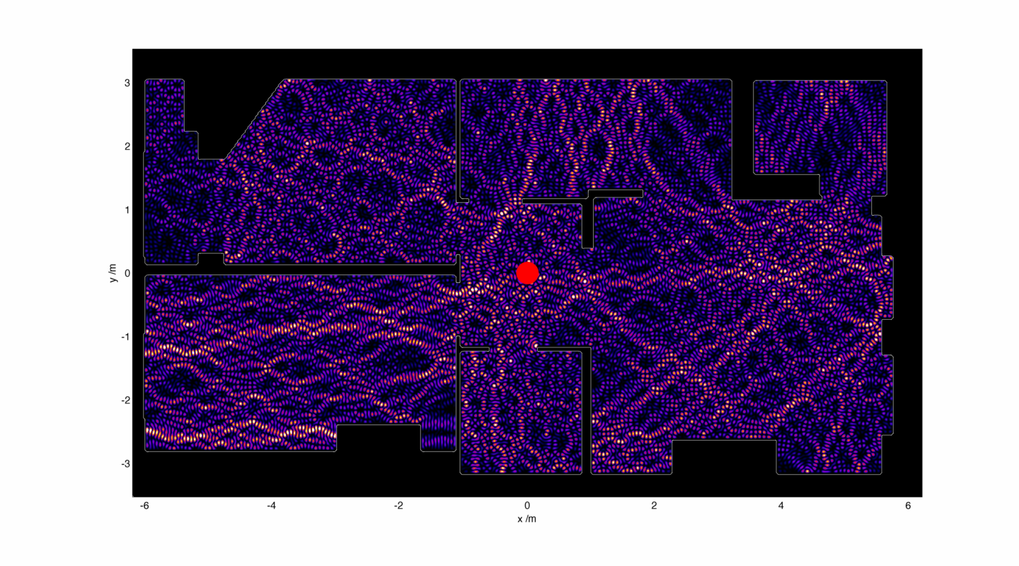
As suggested by a helpful commenter, I tried adding in an imaginary component of the refractive index for the walls, taken from here. This allows for some absorption in the concrete, and stops the perfect reflections forming a standing wave which almost perfectly cancels everything out. The results look like something I would actually expect:

END UPDATE

It’s quite surprising that the final results should be so sensitive, but given we’re performing a matrix inversion in the solution, the field strength at every position depends on the field strength at every other position. This might seem to be invoking some sort of non-local interaction of the electromagnetic field, but actually its just due to the way we’ve decided to solve the problem.

The Helmholtz equation implicitly assumes a solution independent of time, other than a sinusoidal oscillation. What we end up with is then a system at equilibrium, oscillating back and forth as a trapped standing wave. In effect the antenna has been switched on for an infinite amount of time and all possible reflections, refractions, transmissions etc. have been allowed to happen. There is certainly enough time for all parts of the flat to affect every other part of the flat then, and ‘non-locality’ isn’t an issue. In a practical sense, after a second the electromagnetic waves have had time to zip around the place billions of times and so equilibrium happens extremely quickly.

Now it’s all very well and good to chat about this so glibly, because we’re all physicists and 90% of the time we’re rationalising away difficult-to-do things as ‘obvious’ or ‘trivial’ to avoid doing any work. Unfortunately for me the point of this blog is to do lots of work in my spare time while avoiding doing anything actually useful, so lets see if we can’t have a go at the time-dependent problem. Once we start reintroducing ‘s into the Helmholtz equation it’s actually not an approximation at all any more and we’re back to solving the full set of Maxwell’s equations.

This is exactly what the FDTD technique achieves – Finite Difference Time Domain. The FD means we’re solving equations on a grid, and the TD just makes it all a bit harder. To be specific there is a simple algorithm to march Maxwell’s equations forwards in time, namely

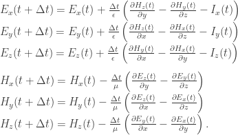
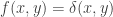
I’ve introduced a current source and the relative permittivity/permeability and such that . We can use all of the machinery mentioned above to discretise the flat layout into a grid, but this time repeatedly apply the above equations. All 6 variables are stored on the grid and updated for every time step. The RAM requirements aren’t so strict in this case which would allow me to model the full flat down to millimetre resolution, but this is just too slow. A full simulation might take all day, and even I can’t justify that. Running one at a longer wavelength 30cm allows me to drop the resolution enough to run a quick simulation before I go to bed.

With the router in approximately the correct place, you can see the radiation initially stream out of the router. There are a few reflections at first, but once the flat has been filled with field it becomes static quite quickly, and settles into an oscillating standing wave. This looks very much like the ‘infinite time’ Helmholtz solution above, albeit at a longer wavelength, and justifies some of the hand-waving ‘intuition’ I tried to fool you with.