By William Cox and Gayan Seneviratna

Do you ever wonder how Grubhub is able to assign you a delivery driver in less than a minute? It’s not magic — it’s because we’re always working to ensure there are just enough drivers in your area for all the orders that people are likely to place in a given moment. Alright, you might say. But how can you be sure of how many orders that’s going to be?

No, it’s not quite that simple.

Today, we’re going to be talking about Demand Forecasting — or, as it’s known at Grubhub, Order Volume Forecasting (OVF). Our goal is to guess how many orders there are going to be in a given area, over a half-hour period. That might seem like a pretty daunting prospect, so let’s start small.

Let’s say you want to guess how many orders there are going to be in Manhattan tomorrow. If that’s the only information you have — a city and a day — you’re going to be shooting in the dark.

But let’s say I told you that yesterday, Manhattanites placed 200 orders. You’d probably guess there’d be around 200 orders again tomorrow. Or maybe you know that tomorrow is Friday, and you know that people order more on Fridays. Maybe you’d increase your guess to 300.

Congratulations, you’ve just performed your first volume forecast! That’s essentially what we do here at Grubhub: use historical order volume, combined with additional predictors, to create accurate and flexible forecasts for our business.

The Data

In practice, we work with much more information than just yesterday’s orders. Our forecasting is built on the entire history of Grubhub orders. In order to understand our data, it’s helpful to take a step back and see what order volume data looks like.

In a standard statistics problem, your unit of analysis (i.e., the thing you care about) is independently and identically distributed, or IID. For example, if you were trying to build a model relating ingredients to food names, your data might look like the following. Above is your data table, and below are your values.

IID means that the order of the rows doesn’t matter. If you guessed that the second item was fondue, it would not affect whether or not the fourth was chimichangas. You could also say that there is no covariance between units of analysis; covariance means that if two values are different in one variable, they’ll be different in others. They vary together.

The data we use in OVF is known as a time-series. It might look something like the following:

Time-series have a time-dependent structure. That is, if you change the order, you change the data’s meaning. Furthermore, the values depend on each other; to refer back to our first example, the number of orders placed tomorrow is related to the number that is placed today.

This dependency means that much of the traditional machine learning methodology needs to be tweaked: everything from building a training data set to your choice of model to generating predictions.

Regions

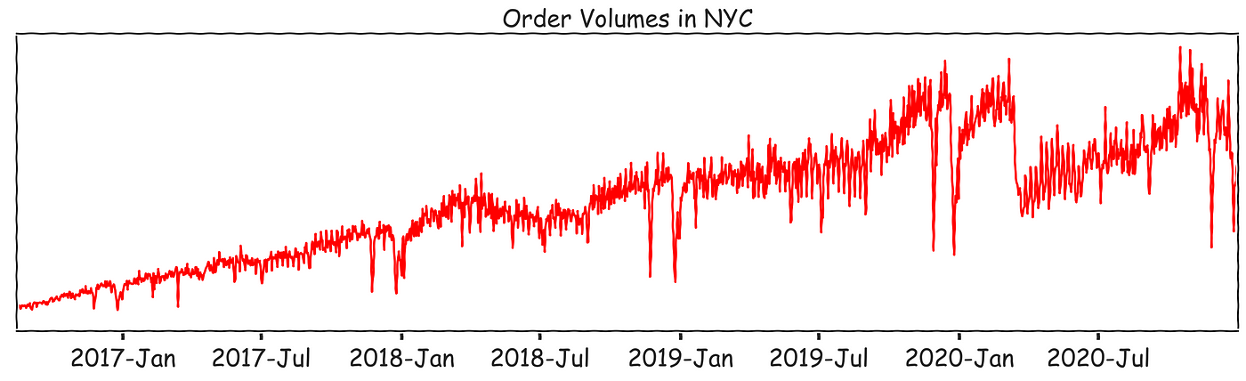
Now that we’ve discussed one time-series, let’s broaden that. Grubhub doesn’t only operate in Manhattan, of course — we have a presence in hundreds of different US markets. These regions are all sized and shaped by customer behavior. Customer behavior varies from market to market. As a result, time-series across these regions all look very different.

Some regions have only a few orders a day, while others have thousands.

Some time-series begin in 2015. Other regions started deliveries as early as last year.

And some regions experience major fluctuations around the holidays, while others hold more steady.

(We realize the y-axes are unlabeled; we can’t share actual business data without hiring you. Nevertheless, these plots demonstrate the variety of our data.)

In order for our forecasts to be successful, we must create a prediction for each time-series. This requires a flexible approach.

Predictors

By now, we’ve established the main input to OVF: hundreds of order volume time-series. But we also make use of other factors, some of which are intrinsic to the time-series itself. For instance, in that first example, we used the day of the week as a predictor.

Other predictors are called “exogenous.” One example of this is whether or not a given day is a holiday. Most diners are eating home-cooked meals on Thanksgiving and Christmas, so it’s important that we predict fewer orders on those days. We use one-hot encoded variables to identify holidays. That is, for a given holiday variable, the value is 0 unless we’re on that date:

The weather would be another example of an exogenous predictor that we consider, as operationalized by variables like snowfall (in inches) or temperature. We then take this information and aggregate it over the time-scale we care about. For instance, the average temperature over a day.

Note that because of the nature of our data, all of these variables are also going to be time-series themselves. Taken together, the data from Manhattan might look as follows:

Modelling Considerations

By now, we understand our data both conceptually and visually. If you haven’t done time series forecasting before, you might be tempted to dive into the problem using a classical research process. Maybe you’d start with linear regression between time and orders, gradually adding additional predictors or complicating the model you’re using.

But as we mentioned earlier, the nature of time-series data, as well as the implied dependence structure, changes how we approach modelling. The following are decisions we must take into account before we begin time-series forecasting.

Backtest Horizons

First we need to divide our data into training and test sets. In a standard modelling scenario, we would randomly sample the data in some ratio. We’d determine model weights based on the first set, then see if they performed well at predicting the values of the second. Let’s see what that looks like for a single time-series:

This is inadvisable, because it isn’t realistic forecasting — you often have all your data up to a certain point and need to predict the next values. The graph above looks more like imputation; we want extrapolation.

The ability to compare against real values is key to training. But how are we supposed to test our model’s ability to predict the future if we don’t know what the future will be?

The solution is backtesting. We begin by selecting a point in our past. We train our models on all data up to a given time point. Then we use the model to forecast a horizon outward, say 14 or 21 days out. Crucially, all of these days are known values in our dataset. Finally, we can calculate performance metrics like MAE or RMSE on the residuals (the differences between the known and forecasted values).

Backtesting allows us to compare various models for accuracy, and decide on the best methods to use in production. We can then use the same procedure from the above plot when we forecast- but we’ll be predicting order volumes that haven’t happened yet.

Extending Predictors

You might have noticed that in the above plot, the weather predictor extends into the training region. When we forecast new values of the target time-series (order volume), we need to have the predictor values ready at that new time point. For holidays, this is easy — you can just look up the desired date. But for variables like weather, we have to rely on weather forecasts, meaning that our forecastalso uses forecasts.

Local vs. Global Models

As mentioned earlier, our data isn’t really a single series, but many different time-series. One of the first questions we ask in time-series modelling is whether we should build our models locally (i.e. one model per region) or globally (across all regions).

Traditionally, local models were the clear choice. These models are able to account for individual patterns in each region. One region might have more orders on July 4th, while another has less. Local models can have appropriately different weights for that predictor. Local models also train relatively quickly — with approximately 2,000 days (5 years) per region, most algorithms can optimize weights in less than a minute.

Global models are meant to forecast the future of any time-series in a dataset, because they are trained on all the series in that dataset. This approach has its advantages: the model may be able to learn overall trends in data, like how regions generally react to offered promotions or discounts. This advantage has often been eclipsed by the specificity of local models. However, recent advances in Deep Learning have allowed for better global models. Examples include DeepAR and Transformer models.

Autoregression vs. Time-Indexed Predictors

Generally speaking, there are two ways we account for the time-dependent nature of time-series data.

The first method is autoregression. Autoregression(AR) refers to the use of recent past values to forecast. For example, a simple AR model might forecast that tomorrow’s orders will be the average of today’s and yesterday’s. The relationships used in AR can also get more complicated. Moving averages (MA) uses the error from yesterday’s forecast as a predictor for today’s. Autoregressive forecasts have the advantage of being quick to react to recent trends.

The second method is with time-indexed components. The simplest version of this is a delta function (a one-time spike or drop) for exogenous predictors. For example, we might have a component in our model that drops the forecast by 50% on a holiday. More complicated components can be used for long-term trends. For example, orders rise in the winter and drop in the summer. A long-term sinusoidal component can mimic that rise and fall.

Note that these methods are not mutually exclusive. In fact, many of the forecasting models we use at Grubhub employ both autoregressive and time-indexed predictors. This allows our forecasts to be flexible in accounting for market trends.

Control Models

Now, let’s say that one morning our weather database goes down. Or perhaps a global pandemic invalidates many of the long-term patterns our model trains on. You know, things that might happen. Suddenly, our autoregressive and component-based global deep learning models are of little use.

This is why we have simpler back-up models we can rely on. For instance, a model that for each forecasted day calculates a weighted average of the same day for the previous four weeks.

This model is also a baseline for developing new models. If a model we create can’t outperform this naive model, we drop development and move on to the next.

Ensembles

We’ve now discussed many different forecasting models. The ones we use, and their properties, are as follows:

You can see that we have five different models, each used to forecast hundreds of regions. But in the end, we need to have a single value for each region’s forecast. To accomplish that, we rely on a technique known as ensembling.

Perhaps not unsurprisingly, it turns out that when you combine a bunch of models, you tend to outperform any single other model. And that’s exactly what we do — take a simple median of the forecasts from each of these predictors.

To return to our original question — how do we know how many orders there’s going to be in a given area — that’s how! We take that median value and send it to our coworkers in scheduling, who, in turn, make sure there are enough Grubhub drivers in that area to meet demand.

What’s Up Next?

At this point, you should have a pretty good conceptual understanding of how we manage order volume forecasting: what the data looks like, how the models work, and how they combine to get our predictions.

Time series forecasting is a powerful methodology, with applications across industries. In healthcare, it can help track biometric trajectories. Environmental scientists can use it to predict changes to the climate. Quants in the finance industry use it for investments. And as more actors enter the space, research has continued making the models better and better.

But that’s only part of the story. It’s great to have a model, but how do we use it?

Stay tuned for part 2!