OpenCV中的图像变换——傅里叶变换

这篇博客将介绍OpenCV中的图像变换，包括用Numpy、OpenCV计算图像的傅里叶变换，以及傅里叶变换的一些应用；

2D Discrete Fourier Transform (DFT)二维离散傅里叶变换
Fast Fourier Transform (FFT) 快速傅里叶变换

傅立叶变换用于分析各种滤波器的频率特性。对于图像采用二维离散傅立叶变换（DFT）求频域。一种称为快速傅立叶变换（FFT）的快速算法用于DFT的计算。

• OpenCV使用cv2.dft()、cv2.idft() 实现傅里叶变换，效率更高一些（比OpenCV快3倍）
• Numpy使用np.ifft2() 、np.fft.ifftshift() 实现傅里叶变换，使用更友好一些；

1. 效果图

灰度图 VS 傅里叶变换效果图如下：
可以看到白色区域大多在中心，显示低频率的内容比较多。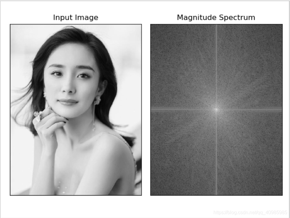

傅里叶变换去掉低频内容后效果图如下：

可以看到使用矩形滤波后，效果并不好，有波纹的振铃效果；用高斯滤波能好点；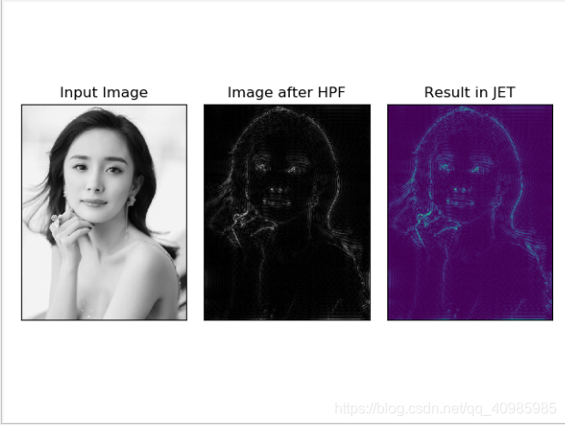

傅里叶变换去掉高频内容后效果图如下：
删除图像中的高频内容，即将LPF应用于图像，它实际上模糊了图像。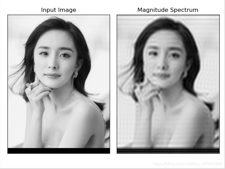

各滤波器是 HPF（High Pass Filter）还是 LPF（Low Pass Filter），一目了然：
拉普拉斯是高频滤波器；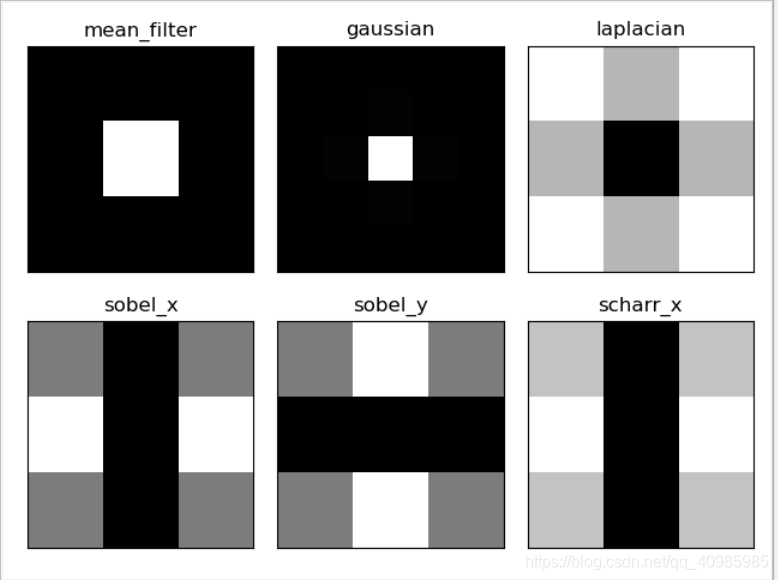

• DFT的性能优化：在一定的阵列尺寸下，DFT计算的性能较好。当数组大小为2的幂时，速度最快。大小为2、3和5的乘积的数组也可以非常有效地处理。

为达到最佳性能，可以通过OpenCV提供的函数cv2.getOptimalDFTSize() 寻找最佳尺寸。
然后将图像填充成最佳性能大小的阵列，对于OpenCV，必须手动填充零。但是对于Numpy，可以指定FFT计算的新大小,会自动填充零。

通过使用最优阵列，基本能提升4倍的效率。而OpenCV本身比Numpy效率快近3倍；

拉普拉斯是高通滤波器（High Pass Filter）

3.1 Numpy实现傅里叶变换

# 傅里叶变换

import cv2
import numpy as np
from matplotlib import pyplot as plt

img = cv2.imread('ym3.jpg', 0)

# 使用Numpy实现傅里叶变换：fft包
# fft.fft2() 进行频率变换
# 参数1：输入图像的灰度图
# 参数2：>输入图像 用0填充；  <输入图像 剪切输入图像； 不传递 返回输入图像
f = np.fft.fft2(img)

# 一旦得到结果，零频率分量（直流分量）将出现在左上角。
# 如果要将其置于中心，则需要使用np.fft.fftshift()将结果在两个方向上移动。
# 一旦找到了频率变换，就能找到幅度谱。
fshift = np.fft.fftshift(f)
magnitude_spectrum = 20 * np.log(np.abs(fshift))

plt.subplot(121), plt.imshow(img, cmap='gray')
plt.title('Input Image'), plt.xticks([]), plt.yticks([])
plt.subplot(122), plt.imshow(magnitude_spectrum, cmap='gray')
plt.title('Magnitude Spectrum'), plt.xticks([]), plt.yticks([])
plt.show()

# 找到了频率变换，就可以进行高通滤波和重建图像，也就是求逆DFT
rows, cols = img.shape
crow, ccol = rows // 2, cols // 2
fshift[crow - 30:crow + 30, ccol - 30:ccol + 30] = 0
f_ishift = np.fft.ifftshift(fshift)
img_back = np.fft.ifft2(f_ishift)
img_back = np.abs(img_back)

# 图像渐变章节学习到：高通滤波是一种边缘检测操作。这也表明大部分图像数据存在于频谱的低频区域。
# 仔细观察结果可以看到最后一张用JET颜色显示的图像，有一些瑕疵（它显示了一些波纹状的结构，这就是所谓的振铃效应。）
# 这是由于用矩形窗口mask造成的，掩码mask被转换为sinc形状，从而导致此问题。所以矩形窗口不用于过滤，更好的选择是高斯mask。）
plt.subplot(131), plt.imshow(img, cmap='gray')
plt.title('Input Image'), plt.xticks([]), plt.yticks([])
plt.subplot(132), plt.imshow(img_back, cmap='gray')
plt.title('Image after HPF'), plt.xticks([]), plt.yticks([])
plt.subplot(133), plt.imshow(img_back)
plt.title('Result in JET'), plt.xticks([]), plt.yticks([])

plt.show()

3.2 OpenCV实现傅里叶变换

import cv2
import numpy as np
from matplotlib import pyplot as plt

img = cv2.imread('ym3.jpg', 0)
rows, cols = img.shape
print(rows, cols)

# 计算DFT效率最佳的尺寸
nrows = cv2.getOptimalDFTSize(rows)
ncols = cv2.getOptimalDFTSize(cols)
print(nrows, ncols)

nimg = np.zeros((nrows, ncols))
nimg[:rows, :cols] = img
img = nimg

# OpenCV计算快速傅里叶变换，输入图像应首先转换为np.float32，然后使用函数cv2.dft()和cv2.idft()。
# 返回结果与Numpy相同，但有两个通道。第一个通道为有结果的实部，第二个通道为有结果的虚部。
dft = cv2.dft(np.float32(img), flags=cv2.DFT_COMPLEX_OUTPUT)
dft_shift = np.fft.fftshift(dft)

magnitude_spectrum = 20 * np.log(cv2.magnitude(dft_shift[:, :, 0], dft_shift[:, :, 1]))

plt.subplot(121), plt.imshow(img, cmap='gray')
plt.title('Input Image'), plt.xticks([]), plt.yticks([])
plt.subplot(122), plt.imshow(magnitude_spectrum, cmap='gray')
plt.title('Magnitude Spectrum'), plt.xticks([]), plt.yticks([])
plt.show()

rows, cols = img.shape
crow, ccol = rows // 2, cols // 2

# 首先创建一个mask，中心正方形为1，其他均为0
# 如何删除图像中的高频内容，即我们将LPF应用于图像。它实际上模糊了图像。
# 为此首先创建一个在低频时具有高值的掩码，即传递LF内容，在HF区域为0。
mask = np.zeros((rows, cols, 2), np.uint8)
mask[crow - 30:crow + 30, ccol - 30:ccol + 30] = 1

# 应用掩码Mask和求逆DTF
fshift = dft_shift * mask
f_ishift = np.fft.ifftshift(fshift)
img_back = cv2.idft(f_ishift)
img_back = cv2.magnitude(img_back[:, :, 0], img_back[:, :, 1])

plt.subplot(121), plt.imshow(img, cmap='gray')
plt.title('Input Image'), plt.xticks([]), plt.yticks([])
plt.subplot(122), plt.imshow(img_back, cmap='gray')
plt.title('Magnitude Spectrum'), plt.xticks([]), plt.yticks([])
plt.show()

3.3 HPF or LPF？

import cv2
import numpy as np
from matplotlib import pyplot as plt

# 简单的均值滤波
mean_filter = np.ones((3, 3))

# 构建高斯滤波
x = cv2.getGaussianKernel(5, 10)
gaussian = x * x.T

# 不同的边缘检测算法Scharr-x方向
scharr = np.array([[-3, 0, 3],
                   [-10, 0, 10],
                   [-3, 0, 3]])
# Sobel_x
sobel_x = np.array([[-1, 0, 1],
                    [-2, 0, 2],
                    [-1, 0, 1]])
# Sobel_y
sobel_y = np.array([[-1, -2, -1],
                    [0, 0, 0],
                    [1, 2, 1]])
# 拉普拉斯
laplacian = np.array([[0, 1, 0],
                      [1, -4, 1],
                      [0, 1, 0]])

filters = [mean_filter, gaussian, laplacian, sobel_x, sobel_y, scharr]
filter_name = ['mean_filter', 'gaussian', 'laplacian', 'sobel_x', \
               'sobel_y', 'scharr_x']
fft_filters = [np.fft.fft2(x) for x in filters]
fft_shift = [np.fft.fftshift(y) for y in fft_filters]
mag_spectrum = [np.log(np.abs(z) + 1) for z in fft_shift]

for i in range(6):
    plt.subplot(2, 3, i + 1), plt.imshow(mag_spectrum[i], cmap='gray')
    plt.title(filter_name[i]), plt.xticks([]), plt.yticks([])

plt.show()

• https://docs.opencv.org/3.0-beta/doc/py_tutorials/py_imgproc/py_transforms/py_fourier_transform/py_fourier_transform.html#fourier-transform