潜在语义分析LSA初探

什么是潜在语义分析LSA？

潜在语义分析（Latent Semantic Analysis），是语义学的一个新的分支。传统的语义学通常研究字、词的含义以及词与词之间的关系，如同义，近义，反义等等。潜在语义分析探讨的是隐藏在字词背后的某种关系，这种关系不是以词典上的定义为基础，而是以字词的使用环境作为最基本的参考。这种思想来自于心理语言学家。他们认为，世界上数以百计的语言都应该有一种共同的简单的机制，使得任何人只要是在某种特定的语言环境下长大都能掌握那种语言。在这种思想的指导下，人们找到了一种简单的数学模型，这种模型的输入是由任何一种语言书写的文献构成的文库，输出是该语言的字、词的一种数学表达（向量）。字、词之间的关系乃至任何文章片断之间的含义的比较就由这种向量之间的运算产生。

向量空间模型是信息检索中最常用的检索方法，其检索过程是，将文档集D中的所有文档和查询都表示成以单词为特征的向量，特征值为每个单词的TF-IDF值，然后使用向量空间模型(亦即计算查询q的向量和每个文档$d_i$的向量之间的相似度)来衡量文档和查询之间的相似度，从而得到和给定查询最相关的文档。向量空间模型简单的基于单词的出现与否以及TF-IDF等信息来进行检索，但是“说了或者写了哪些单词”和“真正想表达的意思”之间有很大的区别，其中两个重要的阻碍是单词的多义性(polysems)和同义性(synonymys)。

• 多义性指的是一个单词可能有多个意思，比如Apple，既可以指水果苹果，也可以指苹果公司
• 同义性指的是多个不同的词可能表示同样的意思，比如search和find。

同义词和多义词的存在使得单纯基于单词的检索方法(比如向量空间模型等)的检索精度受到很大影响。总而言之，在基于单词的检索方法中，同义词会降低检索算法的召回率(Recall)，而多义词的存在会降低检索系统的准确率(Precision)。

LSA和传统向量空间模型(vector space model)一样使用向量来表示词(terms)和文档(documents)，并通过向量间的关系(如夹角)来判断词及文档间的关系；不同的是，LSA 将词和文档映射到潜在语义空间，从而去除了原始向量空间中的一些“噪音”，提高了信息检索的精确度。如果两个单词之间有很强的相关性，那么当一个单词出现时，往往意味着另一个单词也应该出现(同义词)；反之，如果查询语句或者文档中的某个单词和其他单词的相关性都不大，那么这个词很可能表示的是另外一个意思(比如在讨论互联网的文章中，Apple更可能指的是Apple公司，而不是水果)。

LSA工具：

• 2009年：Gensim
• 2015年：fastText
• 2016年：text2Vec

潜在语义分析LSA原理

假设有 n 篇文档，这些文档中的单词总数为 m (可以先进行分词、去词根、去停止词操作),我们可以用一个 m∗n 的矩阵 X 来表示这些文档，这个矩阵的每个元素 $X_{ij}$ 表示第 i 个单词在第 j 篇文档中出现的次数(也可用tf-idf值)。下文例子中得到的矩阵见下图。

LSA试图将原始矩阵降维到一个潜在的概念空间（维度不超过n），然后每个单词或文档都可以用该空间下的一组权值向量（也可认为是坐标）来表示，这些权值反应了与对应的潜在概念的关联程度的强弱。这个降维是通过对该矩阵进行奇异值分解(SVD, singular value decomposition)做到的，计算其用三个矩阵的乘积表示的等价形式，如下：

LSA的数学原理是矩阵分解（奇异值分解SVD），本质是线性变换（把文本从单词向量空间映射到语义向量空间，词->语义）

潜在语义分析LSA优缺点

LSA的优点：

• 低维空间表示可以刻画同义词，同义词会对应着相同或相似的主题。
• 降维可去除部分噪声，是特征更鲁棒。
• 充分利用冗余数据。
• 无监督/完全自动化。
• 与语言无关。

LSA的缺点：

• LSA可以处理向量空间模型无法解决的一义多词(synonymy)问题，但不能解决一词多义(polysemy)问题。因为LSA将每一个词映射为潜在语义空间中的一个点，也就是说一个词的多个意思在空间中对于的是同一个点，并没有被区分。
• SVD的优化目标基于L-2 norm 或者 Frobenius Norm 的，这相当于隐含了对数据的高斯分布假设。而 term 出现的次数是非负的，这明显不符合 Gaussian 假设，而更接近 Multi-nomial 分布。
• 特征向量的方向没有对应的物理解释。
• SVD的计算复杂度很高，而且当有新的文档来到时，若要更新模型需重新训练。
• 没有刻画term出现次数的概率模型。
• 对于count vectors 而言，欧式距离表达是不合适的（重建时会产生负数）。
• 维数的选择是ad-hoc的。
• LSA具有词袋模型的缺点，即在一篇文章，或者一个句子中忽略词语的先后顺序。
• LSA的概率模型假设文档和词的分布是服从联合正态分布的，但从观测数据来看是服从泊松分布的。因此LSA算法的一个改进PLSA使用了多项分布，其效果要好于LSA。

潜在语义分析LSA代码示例

# -*- coding: utf-8 -*-
from numpy import zeros
from scipy.linalg import svd
from math import log
import numpy as np
import seaborn as sns
import matplotlib.pyplot as plt
import pandas as pd


class LSA(object):
    """
    定义LSA类，w_dict字典用来记录词的个数，d_count用来记录文档号。
    """
    def __init__(self, stop_words, ignore_chars):
        self.stop_words = stop_words
        self.ignore_chars = ignore_chars
        self.w_dict = {}
        self.d_count = 0

    def parse(self, doc):
        """
        把文档分词，并滤除停用词和标点，剩下的词会把其出现的文档号填入到w_dict中去，
        例如，词book出现在标题3和4中，则我们有self.w_dict[‘book’] = [3, 4]。相当于建了一下倒排。
        """
        words = doc.split()
        for w in words:
            w = w.lower().translate(self.ignore_chars)
            if w in self.stop_words:
                pass
            elif w in self.w_dict:
                self.w_dict[w].append(self.d_count)
            else:
                self.w_dict[w] = [self.d_count]
        self.d_count += 1

    def build(self):
        """
        建立索引词文档矩阵
        所有的文档被解析之后，所有出现的词（也就是词典的keys）被取出并且排序。建立一个矩阵，其行数是词的个数，列数是文档个数。
        最后，所有的词和文档对所对应的矩阵单元的值被统计出来。
        """
        self.keys = [k for k in self.w_dict.keys() if len(self.w_dict[k]) > 1]
        self.keys.sort()
        self.A = zeros([len(self.keys), self.d_count])
        for i, k in enumerate(self.keys):
            for d in self.w_dict[k]:
                self.A[i, d] += 1

    def print_A(self):
        """
        打印出索引词文档矩阵。
        """
        print(self.A)

    def TF_IDF(self):
        """
        用TF-IDF替代简单计数
        在复杂的LSA系统中，为了重要的词占据更重的权重，原始矩阵中的计数往往会被修改。
        最常用的权重计算方法就是TF-IDF（词频-逆文档频率）。基于这种方法，我们把每个单元的数值进行修改。
        wordsPerDoc 就是矩阵每列的和,也就是每篇文档的词语总数。DocsPerWord 利用asarray方法创建一个0、1数组（也就是大于0的数值会被归一到1），然后每一行会被加起来，从而计算出每个词出现在了多少文档中。最后，我们对每一个矩阵单元计算TFIDF公式
        """
        words_per_doc = np.sum(self.A, axis=0)
        docs_per_word = np.sum(np.asarray(self.A > 0, 'i'), axis=1)
        rows, cols = self.A.shape
        for i in range(rows):
            for j in range(cols):
                self.A[i, j] = (self.A[i, j] / words_per_doc[j]) * log(float(cols) / docs_per_word[i])

    def calc_SVD(self):
        """
        建立完词文档矩阵以后，用奇异值分解（SVD）分析这个矩阵。
        SVD非常有用的原因是，它能够找到我们矩阵的一个降维表示，他强化了其中较强的关系并且扔掉了噪音（这个算法也常被用来做图像压缩）。
        换句话说，它可以用尽可能少的信息尽量完善的去重建整个矩阵。为了做到这点，它会扔掉无用的噪音，强化本身较强的模式和趋势。
        利用SVD的技巧就是去找到用多少维度（概念）去估计这个矩阵。太少的维度会导致重要的模式被扔掉，反之维度太多会引入一些噪音。
        代码中降到了3维
        """
        self.U, self.S, self.Vt = svd(self.A)
        target_dimension = 3
        self.U2 = self.U[0:, 0:target_dimension]
        self.S2 = np.diag(self.S[0:target_dimension])
        self.Vt2 = self.Vt[0:target_dimension, 0:]
        print("U:\n", self.U2)
        print("S:\n", self.S2)
        print("Vt:\n", self.Vt2)

    def plot_singular_values_bar(self):
        """
        为了去选择一个合适的维度数量，我们可以做一个奇异值平方的直方图。它描绘了每个奇异值对于估算矩阵的重要度。
        下图是我们这个例子的直方图。（每个奇异值的平方代表了重要程度，下图应该是归一化后的结果）
        """
        y_value = (self.S * self.S) / sum(self.S * self.S)
        x_value = range(len(y_value))
        plt.bar(x_value, y_value, alpha=1, color='g', align="center")
        plt.autoscale()
        plt.xlabel("Singular Values")
        plt.ylabel("Importance")
        plt.title("The importance of Each Singular Value")
        plt.show()

    def plot_singular_heatmap(self):
        """
        用颜色聚类
        我们可以把数字转换为颜色。例如，下图表示了文档矩阵3个维度的颜色分布。除了蓝色表示负值，红色表示正值，它包含了和矩阵同样的信息。
        """
        labels = ["T1", "T2", "T3", "T4", "T5", "T6", "T7", "T8", "T9"]
        rows = ["Dim1", "Dim2", "Dim3"]
        self.Vt_df_norm = pd.DataFrame(self.Vt2 * (-1))
        self.Vt_df_norm.columns = labels
        self.Vt_df_norm.index = rows
        sns.set(font_scale=1.2)
        ax = sns.heatmap(self.Vt_df_norm, cmap=plt.cm.bwr, linewidths=.1, square=2)
        ax.xaxis.tick_top()
        plt.xlabel("Book Title")
        plt.ylabel("Dimensions")
        plt.show()


if __name__ == '__main__':
    # 待处理的文档
    titles = [
        "The Neatest Little Guide to Stock Market Investing",
        "Investing For Dummies, 4th Edition",
        "The Little Book of Common Sense Investing: The Only Way to Guarantee Your Fair Share of Stock Market Returns",
        "The Little Book of Value Investing",
        "Value Investing: From Graham to Buffett and Beyond",
        "Rich Dad's Guide to Investing: What the Rich Invest in, That the Poor and the Middle Class Do Not!",
        "Investing in Real Estate, 5th Edition",
        "Stock Investing For Dummies",
        "Rich Dad's Advisors: The ABC's of Real Estate Investing: The Secrets of Finding Hidden Profits Most Investors Miss"
    ]
    # 定义停止词
    stopwords = ['and', 'edition', 'for', 'in', 'little', 'of', 'the', 'to']
    # 定义要去除的标点符号
    ignore_chars = ''',:'!'''

    mylsa = LSA(stopwords, ignore_chars)
    for t in titles:
        mylsa.parse(t)
    mylsa.build()
    mylsa.print_A()
    mylsa.TF_IDF()
    mylsa.print_A()
    mylsa.calc_SVD()
    mylsa.plot_singular_values_bar()
    mylsa.plot_singular_heatmap()

在 sklearn 中，LSA可以更加方便的实现：

import pandas as pd
import matplotlib.pyplot as plt
from nltk.corpus import stopwords
from sklearn.feature_extraction.text import TfidfVectorizer
from sklearn.datasets import fetch_20newsgroups
from sklearn.decomposition import TruncatedSVD
import umap

dataset = fetch_20newsgroups(shuffle=True, random_state=1, remove=('headers', 'footers', 'quotes'))
documents = dataset.data
print(len(documents))
print(dataset.target_names)

news_df = pd.DataFrame({'document': documents})

# remove everything except alphabets`
news_df['clean_doc'] = news_df['document'].replace("[^a-zA-Z]", " ")

# remove short words
news_df['clean_doc'] = news_df['clean_doc'].apply(lambda x: ' '.join([w for w in x.split() if len(w) > 3]))

# make all text lowercase-
news_df['clean_doc'] = news_df['clean_doc'].apply(lambda x: x.lower())

# tokenization
tokenized_doc = news_df['clean_doc'].apply(lambda x: x.split())

# remove stop-words
stop_words = stopwords.words('english')
tokenized_doc = tokenized_doc.apply(lambda x: [item for item in x if item not in stop_words])

# de-tokenization
detokenized_doc = []
for i in range(len(news_df)):
    t = ' '.join(tokenized_doc[i])
    detokenized_doc.append(t)

news_df['clean_doc'] = detokenized_doc

vectorizer = TfidfVectorizer(stop_words='english', max_features=1000, max_df=0.5, smooth_idf=True)
X = vectorizer.fit_transform(news_df['clean_doc'])
print(X.shape)

# SVD represent documents and terms in vectors
svd_model = TruncatedSVD(n_components=20, algorithm='randomized', n_iter=100, random_state=122)
svd_model.fit(X)
print(len(svd_model.components_))

terms = vectorizer.get_feature_names()
for i, comp in enumerate(svd_model.components_):
    terms_comp = zip(terms, comp)
    sorted_terms = sorted(terms_comp, key=lambda x: x[1],reverse=True)[:7]
    sorted_terms_words = [t[0] for t in sorted_terms]
    print("Topic " + str(i) + ": " + str(sorted_terms_words))

X_topics = svd_model.fit_transform(X)
embedding = umap.UMAP(n_neighbors=150, min_dist=0.5, random_state=12).fit_transform(X_topics)
plt.figure(figsize=(7, 5))
plt.scatter(embedding[:, 0], embedding[:, 1], c=dataset.target, s=10, edgecolor='none')
plt.show()

潜在语义分析实战：基于LSA的情感分类

数据集：Amazon.com 50万点评数据

字段说明：

• Id：自增长ID，无含义
• ProductId：产品ID
• UserId：会员ID
• ProfileName：会员昵称
• HelpfulnessNumerator：评价点评有用数量
• HelpfulnessDenominator：评价点评总数
• Score：点评分
• Time：点评时间
• Summary：综合评价
• Text：点评详情

这里只会用到2个字段：Score和Text。Score：总共5分，我们将1分、2分的看作是负面评论。4分、5分的看作是正面评论。将3分的中性评论直接删除。

加载Python包：

import numpy as np
import pandas as pd
from sklearn.feature_extraction.text import TfidfVectorizer
from sklearn.model_selection import train_test_split
from sklearn.feature_extraction.text import CountVectorizer
from sklearn.ensemble import RandomForestClassifier
from sklearn.pipeline import Pipeline
from sklearn.metrics import accuracy_score
from sklearn.metrics import classification_report
from sklearn.feature_selection import chi2
import matplotlib.pyplot as plt

准备数据：

df = pd.read_csv('Reviews.csv')
df.dropna(inplace=True)
df[df['Score'] != 3]
df['Positivity'] = np.where(df['Score'] > 3, 1, 0)
X = df['Text']
y = df['Positivity']
X_train, X_test, y_train, y_test = train_test_split(X, y, test_size=0.25, random_state=0)
print("Train set has total {0} entries with {1:.2f}% negative, {2:.2f}% positive".format(
    len(X_train),
    (len(X_train[y_train == 0]) / (len(X_train) * 1.)) * 100,
    (len(X_train[y_train == 1]) / (len(X_train) * 1.)) * 100)
)

我们可以看到正面点评和负面点评并不均衡。Train set has total 426308 entries with 21.91% negative, 78.09% positive。情感分类我们使用决策树算法（随机森林）并设置class_weight=balanced

定义一个计算准确率的函数：

def accuracy_summary(pipeline, X_train, y_train, X_test, y_test):
    sentiment_fit = pipeline.fit(X_train, y_train)
    y_pred = sentiment_fit.predict(X_test)
    accuracy = accuracy_score(y_test, y_pred)
    print("accuracy score: {0:.2f}%".format(accuracy * 100))
    return accuracy

在进行LSA的时，如果如果不做限制，我们会使用Text中所有出现过的单词作为特征，这样的计算量和效果并不佳。取而代之的是我们的获取TOP的单词作为特征。我们分别使用10000,20000,30000做测试：

cv = CountVectorizer()
rf = RandomForestClassifier(class_weight="balanced")
n_features = np.arange(10000, 30001, 10000)


def nfeature_accuracy_checker(vectorizer=cv, n_features=n_features, stop_words=None, ngram_range=(1, 1), classifier=rf):
    result = []
    print(classifier)
    for n in n_features:
        vectorizer.set_params(stop_words=stop_words, max_features=n, ngram_range=ngram_range)
        checker_pipeline = Pipeline([
            ('vectorizer', vectorizer),
            ('classifier', classifier)
        ])
        print("Test result for {} features".format(n))
        nfeature_accuracy = accuracy_summary(checker_pipeline, X_train, y_train, X_test, y_test)
        result.append((n, nfeature_accuracy))
    return result


tfidf = TfidfVectorizer()
feature_result_tgt = nfeature_accuracy_checker(vectorizer=tfidf, ngram_range=(1, 3))

我们可以看到30000特征的时候准确率是最高的。我们可以查看更为详细的指标：

cv = CountVectorizer(max_features=30000, ngram_range=(1, 3))
pipeline = Pipeline([
    ('vectorizer', cv),
    ('classifier', rf)
])
sentiment_fit = pipeline.fit(X_train, y_train)
y_pred = sentiment_fit.predict(X_test)
print(classification_report(y_test, y_pred, target_names=['negative', 'positive']))

使用卡方检验选择特征。我们计算所有特征的卡方得分，并将TOP 20进行可视化。

tfidf = TfidfVectorizer(max_features=30000, ngram_range=(1, 3))
X_tfidf = tfidf.fit_transform(df.Text)
y = df.Positivity
chi2score = chi2(X_tfidf, y)[0]

plt.figure(figsize=(12, 8))
scores = list(zip(tfidf.get_feature_names(), chi2score))
chi2 = sorted(scores, key=lambda x: x[1])
topchi2 = list(zip(*chi2[-20:]))
x = range(len(topchi2[1]))
labels = topchi2[0]
plt.barh(x, topchi2[1], align='center', alpha=0.5)
plt.plot(topchi2[1], x, '-o', markersize=5, alpha=0.8)
plt.yticks(x, labels)
plt.xlabel('$\chi^2$')
plt.show()

潜在语义分析LSA的进化

LSA 方法快速且高效，但它也有一些主要缺点：

• 缺乏可解释的嵌入（我们并不知道主题是什么，其成分可能积极或消极，这一点是随机的）
• 需要大量的文件和词汇来获得准确的结果
• 表征效率低

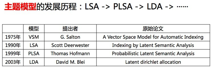
pLSA，即概率潜在语义分析，采取概率方法替代 SVD 以解决问题。其核心思想是找到一个潜在主题的概率模型，该模型可以生成我们在文档-术语矩阵中观察到的数据。特别是，我们需要一个模型 P(D,W)，使得对于任何文档 d 和单词 w，P(d,w) 能对应于文档-术语矩阵中的那个条目。

主题模型的基本假设：每个文档由多个主题组成，每个主题由多个单词组成。pLSA 为这些假设增加了概率自旋：

• 给定文档 d，主题 z 以 P(z|d) 的概率出现在该文档中
• 给定主题 z，单词 w 以 P(w|z) 的概率从主题 z 中提取出来

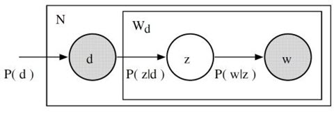
从形式上看，一个给定的文档和单词同时出现的联合概率是：

$$P(D,W)=P(D)\sum_{Z}P(Z|D)P(W|Z)$$

直观来说，等式右边告诉我们理解某个文档的可能性有多大；然后，根据该文档主题的分布情况，在该文档中找到某个单词的可能性有多大。在这种情况下，P(D)、P(Z|D)、和 P(W|Z) 是我们模型的参数。P(D) 可以直接由我们的语料库确定。P(Z|D) 和 P(W|Z) 利用了多项式分布建模，并且可以使用期望最大化算法（EM）进行训练。EM 无需进行算法的完整数学处理，而是一种基于未观测潜变量（此处指主题）的模型找到最可能的参数估值的方法。有趣的是，P(D,W) 可以利用不同的的 3 个参数等效地参数化：

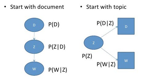
$$P(D,W)=\sum_{Z}P(Z)P(Z|D)P(W|Z)$$

可以通过将模型看作一个生成过程来理解这种等价性。在第一个参数化过程中，我们从概率为 P(d) 的文档开始，然后用 P(z|d) 生成主题，最后用 P(w|z) 生成单词。而在上述这个参数化过程中，我们从 P(z) 开始，再用 P(d|z) 和 P(w|z) 单独生成文档。

这个新参数化方法非常有趣，因为我们可以发现 pLSA 模型和 LSA 模型之间存在一个直接的平行对应关系：

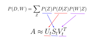
其中，主题 P(Z) 的概率对应于奇异主题概率的对角矩阵，给定主题 P(D|Z) 的文档概率对应于文档-主题矩阵 U，给定主题 P(W|Z) 的单词概率对应于术语-主题矩阵 V。

尽管 pLSA 看起来与 LSA 差异很大、且处理问题的方法完全不同，但实际上 pLSA 只是在 LSA 的基础上添加了对主题和词汇的概率处理。pLSA 是一个更加灵活的模型，但仍然存在一些问题，尤其表现为：

• 因为没有参数来给 P(D) 建模，所以不知道如何为新文档分配概率
• pLSA 的参数数量随着我们拥有的文档数线性增长，因此容易出现过度拟合问题

我们将不会考虑任何 pLSA 的代码，因为很少会单独使用 pLSA。一般来说，当人们在寻找超出 LSA 基准性能的主题模型时，他们会转而使用 LDA 模型。LDA 是最常见的主题模型，它在 pLSA 的基础上进行了扩展，从而解决这些问题。

LDA 即潜在狄利克雷分布，是 pLSA 的贝叶斯版本。它使用狄利克雷先验来处理文档-主题和单词-主题分布，从而有助于更好地泛化。我们可以对狄利克雷分布其做一个简短的概述：即，将狄利克雷视为「分布的分布」。本质上，它回答了这样一个问题：「给定某种分布，我看到的实际概率分布可能是什么样子？」考虑比较主题混合概率分布的相关例子。假设我们正在查看的语料库有着来自 3 个完全不同主题领域的文档。如果我们想对其进行建模，我们想要的分布类型将有着这样的特征：它在其中一个主题上有着极高的权重，而在其他的主题上权重不大。如果我们有 3 个主题，那么我们看到的一些具体概率分布可能会是：

• 混合 X：90% 主题 A，5% 主题 B，5% 主题 C
• 混合 Y：5% 主题 A，90% 主题 B，5% 主题 C
• 混合 Z：5% 主题 A，5% 主题 B，90% 主题 C

如果从这个狄利克雷分布中绘制一个随机概率分布，并对单个主题上的较大权重进行参数化，我们可能会得到一个与混合 X、Y 或 Z 非常相似的分布。我们不太可能会抽样得到这样一个分布：33%的主题 A，33%的主题 B 和 33%的主题 C。本质上，这就是狄利克雷分布所提供的：一种特定类型的抽样概率分布法。我回顾一下 pLSA 的模型：

在 pLSA 中，我们对文档进行抽样，然后根据该文档抽样主题，再根据该主题抽样一个单词。以下是 LDA 的模型：

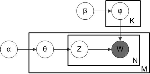
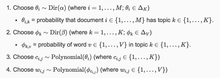
根据狄利克雷分布 Dir(α)，我们绘制一个随机样本来表示特定文档的主题分布或主题混合。这个主题分布记为θ。我们可以基于分布从θ选择一个特定的主题 Z。

接下来，从另一个狄利克雷分布 Dir(𝛽)，我们选择一个随机样本来表示主题 Z 的单词分布。这个单词分布记为φ。从φ中，我们选择单词 w。

从形式上看，从文档生成每个单词的过程如下（注意，该算法使用 c 而不是 z 来表示主题）：

通常而言，LDA 比 pLSA 效果更好，因为它可以轻而易举地泛化到新文档中去。在 pLSA 中，文档概率是数据集中的一个固定点。如果没有看到那个文件，我们就没有那个数据点。然而，在 LDA 中，数据集作为训练数据用于文档-主题分布的狄利克雷分布。即使没有看到某个文件，我们可以很容易地从狄利克雷分布中抽样得来，并继续接下来的操作。

LDA 无疑是最受欢迎（且通常来说是最有效的）主题建模技术。它在 gensim 当中可以方便地使用：

from gensim.corpora.Dictionary import load_from_text, doc2bow
from gensim.corpora import MmCorpus
from gensim.models.ldamodel import LdaModel

document = "This is some document..."

# load id->word mapping (the dictionary)
id2word = load_from_text('wiki_en_wordids.txt')

# load corpus iterator
mm = MmCorpus('wiki_en_tfidf.mm')

# extract 100 LDA topics, updating once every 10,000
lda = LdaModel(corpus=mm, id2word=id2word, num_topics=100, update_every=1, chunksize=10000, passes=1)

# use LDA model: transform new doc to bag-of-words, then apply lda
doc_bow = doc2bow(document.split())
doc_lda = lda[doc_bow]

# doc_lda is vector of length num_topics representing weighted presence of each topic in the doc

通过使用 LDA，我们可以从文档语料库中提取人类可解释的主题，其中每个主题都以与之关联度最高的词语作为特征。例如，主题 2 可以用诸如「石油、天然气、钻井、管道、楔石、能量」等术语来表示。此外，在给定一个新文档的条件下，我们可以获得表示其主题混合的向量，例如，5%的主题 1，70% 的主题 2，10%的主题 3 等。通常来说，这些向量对下游应用非常有用。

深度学习中的 LDA：lda2vec

那么，这些主题模型会将哪些因素纳入更复杂的自然语言处理问题中呢？我们谈到能够从每个级别的文本（单词、段落、文档）中提取其含义是多么重要。在文档层面，我们现在知道如何将文本表示为主题的混合。在单词级别上，我们通常使用诸如 word2vec 之类的东西来获取其向量表征。lda2vec 是 word2vec 和 LDA 的扩展，它共同学习单词、文档和主题向量。

lda2vec 专门在 word2vec 的 skip-gram 模型基础上建模，以生成单词向量。skip-gram 和 word2vec 本质上就是一个神经网络，通过利用输入单词预测周围上下文词语的方法来学习词嵌入。

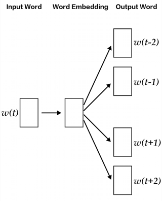
通过使用 lda2vec，我们不直接用单词向量来预测上下文单词，而是使用上下文向量来进行预测。该上下文向量被创建为两个其它向量的总和：单词向量和文档向量。

单词向量由前面讨论过的 skip-gram word2vec 模型生成。而文档向量更有趣，它实际上是下列两个组件的加权组合：

• 文档权重向量，表示文档中每个主题的「权重」（稍后将转换为百分比）
• 主题矩阵，表示每个主题及其相应向量嵌入

文档向量和单词向量协同起来，为文档中的每个单词生成「上下文」向量。lda2vec 的强大之处在于，它不仅能学习单词的词嵌入（和上下文向量嵌入），还同时学习主题表征和文档表征。

参考链接 ：