This article shows how to estimate and visualize a two-dimensional cumulative distribution function (CDF) in SAS. SAS has built-in support for this computation. Although the bivariate CDF is not used as much as the univariate CDF, the bivariate version is still a useful tool in understanding the probable values of a random variate for a two-dimensional distribution.

Recall that the univariate CDF at the value x is the probability that a random observation from a distribution is less than x. In symbols, if X is a random variable, then the distribution function is FX(x)=P(X≤x)FX(x)=P(X≤x). The two-dimensional CDF is similar, but it gives the probability that two random variables are both less than specified values. If X and Y are random variables, the bivariate CDF for the joint distribution is given by FXY(x,y)=P(X≤x and Y≤y)FXY(x,y)=P(X≤xandY≤y).

Univariate estimates of the CDF

Let's start with a one-dimensional example before exploring the topic in higher dimensions. For univariate probability distributions, statisticians use both the density function and the cumulative distribution function. They each contain the same information, and if you know one you can find the other. The cumulative distribution (CDF) of a continuous distribution function is the integral of the probability density function (PDF); the density function is the derivative of the cumulative distribution.

In terms of data analysis, a histogram is an estimate of a density function. So is a kernel density estimate. Consequently, there are three popular methods for estimating a CDF from data:

• The empirical distribution function, which can be computed by using PROC UNIVARIATE. You can get a table of values by using the FREQ option or visualize the curve by using the CDFPLOT statement.
• Add up the values in the bins of a histogram to create an ogive, which is a cumulative histogram. This estimate tends to be coarse unless there are many histogram bins.
• Sum the values of a kernel density estimate to obtain an estimate of the cumulative distribution. You can use the CDF option in PROC KDE to get the cumulative estimates into a SAS data set.

Let's compare the first and last methods to estimate the CDF. For data, use the MPG_City variable from the Sashelp.Cars data.

/* Use PROC UNIVARIATE to compute the empirical CDF from data */
proc univariate data=sashelp.Cars; /* use the FREQ option to get a table */
   var MPG_City;
   cdfplot MPG_City;
   ods select CDFPlot;
   ods output CDFPlot=UNIOut;
run;
 
/* Use PROC KDE to estimate the CDF from a kernel density estimate */
proc kde data=sashelp.Cars;
   univar MPG_City / CDF out=KDEOut;
run;
 
/* combine the estimates and plot on the same graph */
data All;
set UNIOut(rename=(ECDFY=ECDF ECDFX=X))
    KDEOut(rename=(distribution=kerCDF Value=X));
ECDF = ECDF / 100;  /* convert from percent to proportion */
keep X ECDF kerCDF;
run;
 
title "Estimates of CDF";
proc sgplot data=All;
   label X = "MPG_City";
   series x=X y=ECDF / legendlabel="Empirical CDF";
   series x=X y=kerCDF / legendlabel="Kernel CDF";
   yaxis label="Cumulative Distribution" grid;
   xaxis values=(5 to 60 by 5) grid valueshint;
run;

The two estimates are very close. The empirical CDF is more "jagged," whereas the estimate from the kernel density is smoother. You could use either curve to estimate quantiles or probabilities.

Bivariate estimates of the CDF

Now onto the bivariate case. For bivariate data, you cannot use PROC UNIVARIATE (obviously, from the name!), but you can still use PROC KDE. Instead of using the UNIVAR statement, you can use the BIVAR statement to compute a bivariate KDE. Let's look at the joint distribution of the MPG_City and Weight variables in the Sashelp.Cars data:

title;
proc sgplot data=sashelp.Cars;
   scatter x=MPG_City y=Weight;
run;

The scatter plot shows that the density of these points is concentrated near the lower-left corner of the plot. You can use PROC KDE to visualize the density. The PLOTS= option can create a contour plot and a two-dimensional histogram, as follows:

title "2-D Histogram";
proc kde data=sashelp.Cars;
   bivar MPG_City Weight / plots=(Contour Histogram)
         CDF out=KDEOut(rename=(Distribution=kerCDF Value1=X Value2=Y));
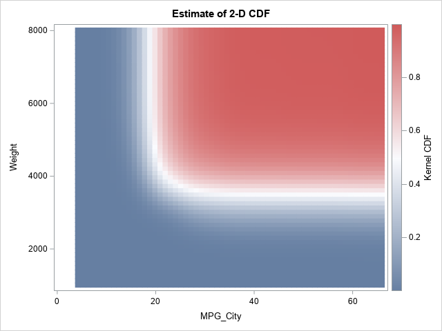
run;

The OUT= option writes a SAS data set that contains the estimates for the density; the CDF option adds the cumulative distribution estimates. The column names are Value1 (for the first variable on the BIVAR statement), Value2 (for the second variable), and Distribution (for the CDF). I have renamed the variables to X, Y, and CDF, but that is not required. You can plot use a heat map (or a contour plot) to visualize the bivariate CDF, as follows:

title "Estimate of 2-D CDF";
proc sgplot data=KDEOut;
   label X="MPG_City" Y="Weight" kerCDF="Kernel CDF";
   heatmapparm x=X y=Y colorresponse=kerCDF; 
run;

The CDF of bivariate normal data

The CDF is not used very often for bivariate data because the density function shows more details. In some sense, all CDFs look similar. In the previous example, the two variables are negatively correlated and are not linearly related. For comparison, the following program uses the RANDNORMAL function in SAS/IML to generate bivariate normal data that has a positive correlation of 0.6. (I have previously shown the empirical CDF for this data, and I have also drawn the graph of the bivariate CDF for the population.) The calls to PROC KDE and PROC SGPLOT are the same as for the previous example:

proc iml;
call randseed(123456);
N = 1e5;                           /* sample size */
rho = 0.6; 
Sigma = ( 1 || rho)//              /* correlation matrix */
        (rho||  1 );
mean = {0 0};
Z = randnormal(N, mean, Sigma);    /* sample from MVN(0, Sigma) */
create BivNorm from Z[c={X Y}];  append from Z;  close;
quit;
 
proc kde data=BivNorm;
   bivar X Y / plots=NONE
         CDF out=KDEOut(rename=(distribution=kerCDF Value1=X Value2=Y));
run;
 
title "Estimate of 2-D Normal CDF";
proc sgplot data=KDEOut aspect=1;
   label kerCDF="Kernel CDF";
   heatmapparm x=X y=Y colorresponse=kerCDF; 
run;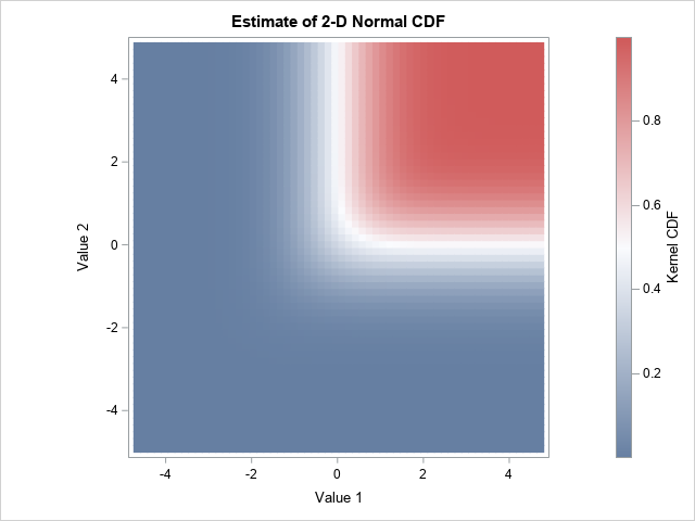

If you compare the bivariate CDF for the Cars data to the CDF for the bivariate normal data, you can see differences in the range of the red region, but the overall impression is the same. The CDF is near 0 in the lower-left corner, near 1 in the upper-right corner, and is approximately 0.5 along an L-shaped curve near the middle of the data. This is the basic shape of a generic 2-D CDF, just as an S-shape or sigmoid-shaped curve is the basic shape of a generic 1-D CDF.

Summary

You can use the CDF option on the BIVAR statement in PROC KDE to obtain an estimate for a bivariate CDF. The estimate is based on a kernel density estimate of the data. You can use the HEATMAPPARM statement in PROC SGPLOT to visualize the CDF surface. If you prefer a contour plot, you can use the graph template language (GTL) to create a contour plot.