Do you know what a copula is? It is a popular way to simulate multivariate correlated data. The literature for copulas is mathematically formidable, but this article provides an intuitive introduction to copulas by describing the geometry of the transformations that are involved in the simulation process. Although there are several families of copulas, this article focuses on the Gaussian copula, which is the simplest to understand.

This article shows the geometry of copulas. This article and its example are based on Chapter 9 of Simulating Data with SAS (Wicklin, 2013). A previous article shows the geometry of the Iman-Conover transformation, which is an alternative way to create simulated data that have a specified rank correlation structure and specified marginal distributions.

Simulate data by using a copula

Recall that you can use the CDF function to transform any distribution to the uniform distribution. Similarly, you can use the inverse CDF to transform the uniform distribution to any distribution. To simulate correlated multivariate data from a Gaussian copula, follow these three steps:

1. Simulate correlated multivariate normal data from a correlation matrix. The marginal distributions are all standard normal.
2. Use the standard normal CDF to transform the normal marginals to the uniform distribution.
3. Use inverse CDFs to transform the uniform marginals to whatever distributions you want.

The transformation in the second and third steps are performed on the individual columns of a data matrix. The transformations are monotonic, which means that they do not change the rank correlation between the columns. Thus, the final data has the same rank correlation as the multivariate normal data in the first step.

The next sections explore a two-dimensional example of using a Gaussian copula to simulate correlated data where one variable is Gamma-distributed and the other is Lognormally distributed. The article then provides intuition about what a copula is and how to visualize it. You can download the complete SAS program that generates the example and creates the graphs in this article.

A motivating example

Suppose that you want to simulate data from a bivariate distribution that has the following properties:

• The rank correlation between the variables is approximately 0.6.
• The marginal distribution of the first variable, X1, is Gamma(4) with unit scale.
• The marginal distribution of the second variable, X2, is lognormal with parameters μ=0.5 and σ=0.8. That is, log(X2) ~ N(μ, σ).

The hard part of a multivariate simulation is getting the correlation structure correct, so let's start there. It seems daunting to generate a "Gamma-Lognormal distribution" with a correlation of 0.6, but it is straightforward to generate a bivariate NORMAL distribution with that correlation. Let's do that. Then we'll use a series of transformations to transform the normal marginal variables into the distributions that we want while preserving the rank correlation at each step.

Simulate multivariate normal data

The SAS/IML language supports the RANDNORMAL function, which can generate multivariate normal samples, as shown in the following statements:

proc iml;
N = 1e4;
call randseed(12345);
/* 1. Z ~ MVN(0, Sigma) */
Sigma = {1.0  0.6,
         0.6  1.0};
Z = RandNormal(N, {0,0}, Sigma);          /* Z ~ MVN(0, Sigma) */

The matrix Z contains 10,000 observations drawn from a bivariate normal distribution with correlation coefficient ρ=0.6. Because the mean vector is (0,0) and the covariance parameter is a correlation matrix, the marginal distributions are standard normal. The following graph shows a scatter plot of the bivariate normal data along with histograms for each marginal distribution.

Transform marginal distributions to uniform

The first step is to transform the normal marginals into a uniform distribution by using the probability integral transform (also known as the CDF transformation). The columns of Z are standard normal, so Φ(X) ~ U(0,1), where Φ is the cumulative distribution function (CDF) for the univariate normal distribution. In SAS/IML, the CDF function applies the cumulative distribution function to all elements of a matrix, so the transformation of the columns of Z is a one-liner:

/* 2. transform marginal variables to U(0,1) */
U = cdf("Normal", Z);                     /* U_i are correlated U(0,1) variates */

The columns of U are samples from a standard uniform distribution. However, the columns are not independent. Because the normal CDF is a monotonic transformation, it does not change the rank correlation between the columns. That is, the rank correlation of U is the same as the rank correlation of Z:

/* the rank correlations for Z and U are exactly the same */
rankCorrZ = corr(Z, "Spearman")[2]; 
rankCorrU = corr(U, "Spearman")[2]; 
print rankCorrZ rankCorrU;

The following graph shows a scatter plot of the transformed data along with histograms for each marginal distribution. The histograms show that the columns U1 and U2 are uniformly distributed on [0,1]. However, the joint distribution is correlated, as shown in the following scatter plot:

Transform marginal distributions to any distribution

Now comes the magic. One-dimensional uniform variates are useful because you can transform them into any distribution! How? Just apply the inverse cumulative distribution function of whatever distribution you want. For example, you can obtain gamma variates from the first column of U by applying the inverse gamma CDF. Similarly, you can obtain lognormal variates from the second column of U by applying the inverse lognormal CDF. In SAS, the QUANTILE function applies the inverse CDF, as follows:

/* 3. construct the marginals however you wish */
gamma = quantile("Gamma", U[,1], 4);            /* gamma ~ Gamma(alpha=4)   */
LN    = quantile("LogNormal", U[,2], 0.5, 0.8); /* LN ~ LogNormal(0.5, 0.8) */
X = gamma || LN;
 
/* check that the rank correlation still has not changed */
rankCorrX = corr(X, "Spearman")[2]; 
print rankCorrZ rankCorrX;

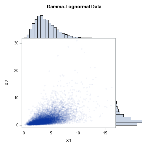
The first column of X is gamma-distributed. The second column of X is lognormally distributed. But because the inverse of a continuous CDF is monotonic, the column transformations do not change the rank correlation between the columns. The following graph shows a scatter plot of the newly transformed data along with histograms for each marginal distribution. The histograms show that the columns X1 and X2 are distributed as gamma and lognormal, respectively. The joint distribution is correlated.

What about the Pearson correlation?

For multivariate normal data, the Pearson correlation is close to the rank correlation. However, that is not true for nonnormal distributions. The CDF and inverse-CDF transformations are nonlinear, so the Pearson correlation is not preserved when you transform the marginal. For example, the following statements compute the Pearson correlation for Z (the multivariate normal data) and for X (the gamma-lognormal data):

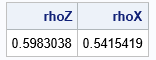
rhoZ = corr(Z, "Pearson")[2];
rhoX = corr(X, "Pearson")[2];
print rhoZ rhoX;

Chapter 9 of Wicklin (2013), discusses the fact that you can adjust the correlation for Z and it will affect the correlation for X in a complicated manner. With a little work, you can choose a correlation for Z that will result in a specified correlation for X. For example, if you want the final Pearson correlation for X to be 0.6, you can use 0.642 as the correlation for Z:

/* re-run the example with new correlation 0.642 */
Sigma = {1.0    0.642,
         0.642  1.0};
newZ = RandNormal(N, {0,0}, Sigma);
newU = cdf("Normal", newZ);           /* columns of U are U(0,1) variates */
gamma = quantile("Gamma", newU[,1], 4);      /* gamma ~ Gamma(alpha=4) */
expo = quantile("Expo", newU[,2]);           /* expo ~ Exp(1)          */
newX = gamma || expo;
 
rhoZ = corr(newZ, "Pearson")[2];
rhoX = corr(newX, "Pearson")[2];
print rhoZ rhoX;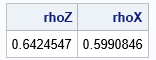

Success! The Pearson correlation between the gamma and lognormal variables is 0.6. In general, this is a complicated process because the value of the initial correlation depends on the target value and on the specific forms of the marginal distributions. Finding the initial value requires finding the root of an equation that involves the CDF and inverse CDF.

Higher dimensional data

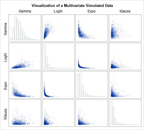
This example in this article generalizes to higher-dimensional data in a natural way. The SAS program that generates the example in this article also includes a four-dimensional example of simulating correlated data. The program simulates four correlated variables whose marginal distributions are distributed as gamma, lognormal, exponential, and inverse Gaussian distributions. The following panel shows the bivariate scatter plots and marginal histograms for this four-dimensional simulated data.

What is a copula?

I've shown many graphs, but what is a copula? The word copula comes from a Latin word (copulare) which means to bind, link, or join. The same Latin root gives us the word "copulate." A mathematical copula is a joint probability distribution that induces a specified correlation structure among independent marginal distributions. Thus, a copula links or joins individual univariate distributions into a joint multivariate distribution that has a specified correlation structure.

Mathematically, a copula is any multivariate cumulative distribution function for which each component variable has a uniform marginal distribution on the interval [0, 1]. That's it. A copula is a cumulative distribution function whose domain is the cube [0,1]d. So the second graph in this article is the graph most nearly related to the copula for the bivariate data, since it shows the relationship between the uniform marginals.

The scatter plot shows the density, not the cumulative distribution. However, you can use the data to estimate the bivariate CDF. The following heat map visualizes the Gaussian copula for the correlation of 0.6:

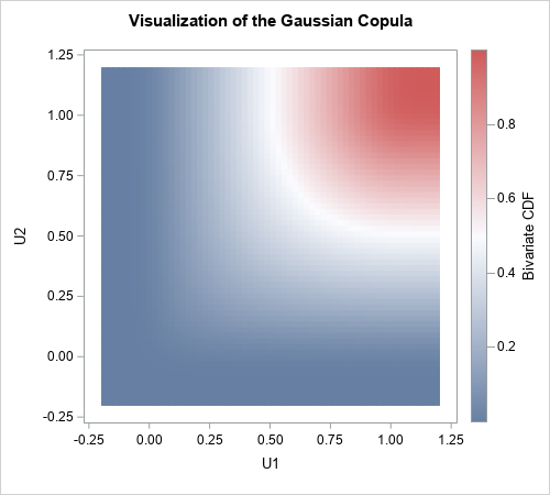
Notice that this function does not depend on the final marginal distributions. It depends only on the multivariate normal distribution and the CDF transformation that produces the uniform marginals. In that sense, the copula captures only the correlation structure, without regard for the final form of the marginal distributions. You can use this same copula for ANY set of marginal distributions because the copula captures the correlation structure independently of the final transformations of the marginals.

Why are copulas important?

A remarkable theorem (Sklar’s theorem) says that every joint distribution can be written as a copula and a set of marginal distributions. If the marginals are continuous, then the copula is unique. Let that sink in for a second: Every continuous multivariate probability distribution can be expressed in terms of its marginal distributions and a copula. Every one. So, if you can understand copulas you can understand all multivariate distributions. Powerful math, indeed!

For simulation studies, you can use the converse of Sklar's theorem, which is also true. Specifically, if you have a set of d uniform random variables and a set of marginal distribution functions, a copula transforms the d components into a d-dimensional probability distribution.

Summary

Copulas are mathematically sophisticated. However, you can use copulas to simulate data without needing to understand all the mathematical details. This article presents an example of using a Gaussian copula to simulate multivariate correlated data. It shows the geometry at each step of the three-step process:

1. Simulate data from a multivariate normal distribution with a known correlation matrix.
2. Use the normal CDF to transform the marginal distributions to uniform.
3. Use inverse CDFs to obtain any marginal distributions that you want.

The result is simulated correlated multivariate data that has the same rank correlation as the original simulated data but has arbitrary marginal distributions.

This article uses SAS/IML to show the geometry of the copula transformations. However, SAS/ETS software provides PROC COPULA, which enables you to perform copula modeling and simulation in a single procedure. A subsequent article shows how to use PROC COPULA.