Heuristic recurrent algorithms for photonic Ising machines

Results

Photonic computational architecture

The proposed architecture of our photonic network is shown in Fig. 1. This photonic network can map arbitrary Ising Hamiltonians described by Eq. (1), with Kii  = 0 (as diagonal terms only contribute to a global offset of the Hamiltonian, see Supplementary Note 1). In the following, we will refer to the eigenvalue decomposition of K as K  = UDU†, where U is a unitary matrix, U† its transpose conjugate, and D a real-valued diagonal matrix. The spin state at time step t, encoded in the phase and amplitude of N parallel photonic signals S(t) ∈ {0, 1}N, first goes through a linear symmetric transformation decomposed in its eigenvalue form 2J = USqα(D)U†, where Sqα(D) is a diagonal matrix derived from D, whose design will be discussed in the next paragraphs. The signal is then fed into nonlinear optoelectronic domain, where it is perturbed by a Gaussian distribution of standard deviation ϕ (simulating noise present in the photonic implementation) and is imparted a nonlinear threshold function Thθ (Thθ(x) = 1 if x > θ, 0 otherwise). The signal is then recurrently fed back to the linear photonic domain, and the process repeats. The static unit transformation between two time steps t and t + 1 of this RNN can be summarized as

where \({\mathcal{N}}(x| \phi )\) denotes a Gaussian distribution of mean x and standard deviation ϕ. We call this algorithm, which is tailored for a photonic implementation, the Photonic Recurrent Ising Sampler (PRIS). The detailed choice of algorithm parameters is described in the Supplementary Note 2.

Fig. 1: Operation principle of the PRIS.

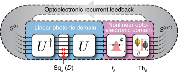
A photonic analog signal, encoding the current spin state S(t), goes through transformations in linear photonic and nonlinear optoelectronic domains. The result of this transformation S(t+1) is recurrently fed back to the input of this passive photonic system.

Full size image

This simple recurrent loop can be readily implemented in the photonic domain. For example, the linear photonic interference unit can be realized with MZI networks34,37,38,39, diffractive optics40,41, ring resonator filter banks42,43,44, and free space lens-SLM-lens systems45,46; the diagonal matrix multiplication Sqα(D) can be implemented with an electro-optical absorber, a modulator or a single MZI34,47,48; the nonlinear optoelectronic unit can be implemented with an optical nonlinearity47,48,49,50,51, or analog/digital electronics52,53,54,55, for instance by converting the optical output to an analog electronic signal, and using this electronic signal to modulate the input56. The implementation of the PRIS on several photonic architectures and the influence of heterogeneities, phase bit precision, and signal to noise ratio on scaling properties are discussed in the Supplementary Note 5. In the following, we will describe the properties of an ideal PRIS and how design imperfections may affect its performance.

General theory of the PRIS dynamics

The long-time dynamics of the PRIS is described by an effective Hamiltonian HL (see refs. 19,58 and Supplementary Note 2). This effective Hamiltonian can be computed by performing the following steps. First, calculate the transition probability of a single spin from Eq. (2). Then, the transition probability from an initial spin state S(t) to the next step S(t+1) can be written as

where \(S,S^{\prime}\) denote arbitrary spin configurations. Let us emphasize that, unlike H(K)(S), the transition Hamiltonian \({H}^{(0)}\left(S| S^{\prime} \right)\) is a function of two spin distributions S and \(S^{\prime}\). Here, β = 1∕(kϕ) is analogous to the inverse temperature from statistical mechanics, where k is a constant, only depending on the noise distribution (see Supplementary Table 1). To obtain Eqs. (3), (4), we approximated the single spin transition probability by a rescaled sigmoid function and have enforced the condition θi = ∑jJij. In the Supplementary Note 2, we investigate the more general case of arbitrary threshold vectors θi and discuss the influence of the noise distribution.

One can easily verify that this transition probability obeys the triangular condition (or detailed balance condition) if J is symmetric Jij = Jji. From there, an effective Hamiltonian HL can be deduced following the procedure described by Peretto58 for distributions verifying the detailed balance condition. The effective Hamiltonian HL can be expanded, in the large noise approximation (ϕ ≫ 1, β ≪ 1), into H2:

Examining Eq. (6), we can deduce a mapping of the PRIS to the general Ising model shown in Eq. (1) since \({H}_{2}=\beta {H}^{({J}^{2})}\). We set the PRIS matrix J to be a modified square-root of the Ising matrix K by imposing the following condition on the PRIS

We add a diagonal offset term αΔ to the eigenvalue matrix D, in order to parametrize the number of eigenvalues remaining after taking the real part of the square root. Since lower eigenvalues tend to increase the energy, they can be dropped out so that the algorithm spans the eigenspace associated with higher eigenvalues. We chose to parametrize this offset as follows: \(\alpha \in {\mathbb{R}}\) is called the eigenvalue dropout level, a hyperparameter to select the number of eigenvalues remaining from the original coupling matrix K, and Δ > 0 is a diagonal offset matrix. For instance, Δ can be defined as the sum of the off-diagonal terms of the Ising coupling matrix Δii = Σj≠i∣Kij∣. The addition of Δ only results in a global offset on the Hamiltonian. The purpose of the Δ offset is to make the matrix in the square root diagonally dominant, thus symmetric positive definite, when α is large and positive. Thus, other definitions of the diagonal offset could be proposed. When α → 0, some lower eigenvalues are dropped out by taking the real part of the square root (see Supplementary Note 3); we show below that this improves the performance of the PRIS. We will specify which definition of Δ is used in our study when α ≠ 0. When choosing this definition of Sqα(D) and operating the PRIS in the large noise limit, we can implement any general Ising model (Eq. (1)) on the PRIS (Eq. (6)).

It has been noted that by setting Sqα(D) = D (i.e., the linear photonic domain matrix amounts to the Ising coupling matrix 2J = K), the free energy of the system equals the Ising free energy at any finite temperature (up to a factor of 2, thus exhibiting the same ground states) in the particular case of associative memory couplings19 with finite number of patterns and in the thermodynamic limit, thus drastically constraining the number of degrees of freedom on the couplings. This regime of operation is a direct modification of the Hopfield network, an energy-based model where the couplings between neurons is equal to the Ising coupling between spins. The essential difference between the PRIS in the configuration Sqα(D) = D and a Hopfield network is that the former relies on synchronous spin updates (all spins are updated at every step, in this so-called Little network14) while the latter relies on sequential spin updates (a single randomly picked spin is updated at every step). The former is better suited for a photonic implementation with parallel photonic networks.

In this regime of operation, the PRIS can also benefit from computational speed-ups, if implemented on a conventional architecture, for instance if the coupling matrix is sparse. However, as has been pointed out in theory19 and by our simulations (see Supplementary Note 4, Supplementary Fig. 7), some additional considerations should be taken into account in order to eliminate non-ergodic behaviors in this system. As the regime of operation described by Eq. (7) is general to any coupling, we will use it in the following demonstrations.

Finding the ground state of Ising models with the PRIS

We investigate the performance of the PRIS on finding the ground state of general Ising problems Eq. (1) with two types of Ising models: MAX-CUT graphs, which can be mapped to an instance of the unweighted MAX-CUT problem9 and all-to-all spin glasses, whose connections are uniformly distributed in [−1, 1] (an example illustration of the latter is shown as an inset in Fig. 2a). Both families of models are computationally NP-hard problems26, thus their computational complexity grows exponentially with the graph order N.

Fig. 2: Scaling performance of the PRIS.

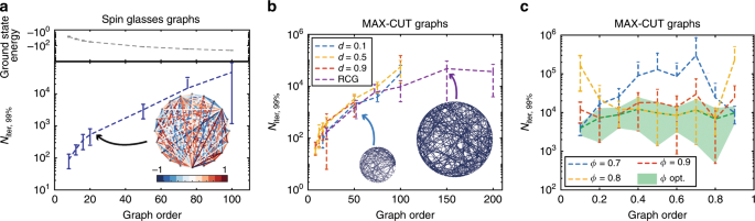
(a, top) Ground state energy versus graph order of random spin glasses. A sample graph is shown as an inset in (a, bottom): a fully-connected spin glass with uniformly-distributed continuous couplings in [−1, 1]. Niter, 99% versus graph size for spin glasses (a, bottom) and MAX-CUT graphs (b). c Niter, 99% versus graph density for MAX-CUT graphs and N = 75. The graph density is defined as d = 2∣E∣∕(N(N − 1)), ∣E∣ being the number of undirected edges. RCG denotes Random Cubic Graphs, for which ∣E∣ = 3N∕2. Ground states are determined with the exact solver BiqMac57 (see Methods section). In this analysis, we set α = 0, and for each set of density and graph order we ran 10 graph instances 1000 times. The number of iterations to find the ground state is measured for each run and Niter, q is defined as the q-th quantile of the measured distribution.

Full size image

The number of steps necessary to find the ground state with 99% probability, Niter, 99% is shown in Fig. 2a–b for these two types of graphs (see definition in Supplementary Note 4 and in the Methods section). As the PRIS can be implemented with high-speed parallel photonic networks, the on-chip real time of a unit step can be less than a nanosecond34,59 (and the initial setup time for a given Ising model is typically of the order of microseconds with thermal phase shifters60). In such architectures, the PRIS would thus find ground states of arbitrary Ising problems with graph orders N ~ 100 within less than a millisecond. We also show that the PRIS can be used as a heuristic ground state search algorithm in regimes where exact solvers typically fail (N ~ 1000) and benchmark its performance against MH and conventional metaheuristics (SA) (see Supplementary Note 6). Interestingly, both classical and quantum optical Ising machines have exhibited limitations in their performance related to the graph density9,61. We observe that the PRIS is roughly insensitive to the graph density, when optimizing the noise level ϕ (see Fig. 2c, shaded green area). A more comprehensive comparison should take into account the static fabrication error in integrated photonic networks34 (see also Supplementary Note 5), even though careful calibration of their control electronics can significantly reduce its impact on the computation62,63.

Influence of the noise and eigenvalue dropout levels

For a given Ising problem, there remain two degrees of freedom in the execution of the PRIS: the noise and eigenvalue dropout levels. The noise level ϕ determines the level of entropy in the Gibbs distribution probed by the PRIS \(p(E)\propto \exp (-\beta (E-\phi S(E)))\), where S(E) is the Boltzmann entropy associated with the energy level E. On the one hand, increasing ϕ will result in an exponential decay of the probability of finding the ground state \(p({H}_{\min },\phi )\). On the other hand, too small a noise level will not satisfy the large noise approximation HL ~ H2 and result in large autocorrelation times (as the spin state could get stuck in a local minimum of the Hamiltonian). Figure 3e demonstrates the existence of an optimal noise level ϕ, minimizing the number of iterations required to find the ground state of a given Ising problem, for various graph sizes, densities, and eigenvalue dropout levels. This optimal noise value can be approximated upon evaluation of the probability of finding the ground state \(p({H}_{\min },\phi )\) and the energy autocorrelation time \({\tau }_{{\rm{auto}}}^{E}\), as the minimum of the following heuristic

which approximates the number of iterations required to find the ground state with probability q (see Fig. 3a–e). In this expression, \({\tau }_{{\rm{eq}}}^{E}(\phi )\) is the energy equilibrium (or burn-in) time. As can be seen in Fig. 3e, decreasing α (and thus dropping more eigenvalues, with the lowest eigenvalues being dropped out first) will result in a smaller optimal noise level ϕ. Comparing the energy landscape for various eigenvalue dropout levels (Fig. 3h) confirms this statement: as α is reduced, the energy landscape is perturbed. However, for the random spin glass studied in Fig. 3f–g, the ground state remains the same down to α = 0. This hints at a general observation: as lower eigenvalues tend to increase the energy, the Ising ground state will in general be contained in the span of eigenvectors associated with higher eigenvalues (see discussion in the Supplementary Note 3). Nonetheless, the global picture is more complex, as the solution of this optimization problem should also enforce the constraint σ ∈ {−1, 1}N. We observe in our simulations that α = 0 yields a higher ground state probability and lower autocorrelation times than α > 0 for all the Ising problems we used in our benchmark. In some sparse models, the optimal value can even be α < 0 (see Supplementary Fig. 3 in the Supplementary Note 4). The eigenvalue dropout is thus a parameter that constrains the dimensionality of the ground state search.

Fig. 3: Influence of noise and eigenvalue dropout levels.

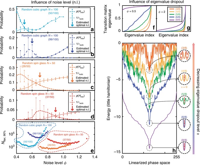
a–d Probability of finding the ground state, and the inverse of the autocorrelation time as a function of noise level ϕ for a sample Random Cubic Graph9 (N = 00, (50/100) eigenvalues (a), (99/100) eigenvalues (b), and a sample spin glass (N = 50, (37/100) eigenvalues (c), (26/100) eigenvalues (d)). The arrows indicate the estimated optimal noise level, from Eq. (8), taking \({\tau }_{{\rm{eq}}}^{E}\) to be constant. For this study we averaged the results of 100 runs of the PRIS with random initial states with error bars representing  ± σ from the mean over the 100 runs. We assumed Δii = ∑jKij. (e): Niter, 90% versus noise level ϕ for these same graphs and eigenvalue dropout levels. f–g Eigenvalues of the transition matrix of a sample spin glass (N = 8) at ϕ = 0.5 (f) and ϕ= 2 (g). h The corresponding energy is plotted for various eigenvalue dropout levels α, corresponding to less than N eigenvalues kept from the original matrix. The inset is a schematic of the relative position of the global minimum when α = 1 (with (8/8) eigenvalues) with respect to nearby local minima when α < 1. For this study we assumed Δii = ∑jKij.

Full size image

The influence of eigenvalue dropout can also be understood from the perspective of the transition matrix. Figure 3f–g shows the eigenvalue distribution of the transition matrix for various noise and eigenvalue dropout levels. As the PRIS matrix eigenvalues are dropped out, the transition matrix eigenvalues become more nonuniform, as in the case of large noise (Fig. 3g). Overall, the eigenvalue dropout can be understood as a means of pushing the PRIS to operate in the large noise approximation, without perturbing the Hamiltonian in such a way that would prevent it from finding the ground state. The improved performance of the PRIS with α ~ 0 hints at the following interpretation: the perturbation of the energy landscape (which affects \(p({H}_{\min })\)) is counterbalanced by the reduction of the energy autocorrelation time induced by the eigenvalue dropout. The existence of these two degrees of freedom suggests a realm of algorithmic techniques to optimize the PRIS operation. One could suggest, for instance, setting α ≈ 0, and then performing an inverse simulated annealing of the eigenvalue dropout level to increase the dimensionality of the ground state search. This class of algorithms could rely on the development of high-speed, low-loss integrated modulators59,64,65,66.

Detecting and characterizing phase transitions with the PRIS

The existence of an effective Hamiltonian describing the PRIS dynamics Eq. (6) further suggests the ability to generate samples of the associated Gibbs distribution at any finite temperature. This is particularly interesting considering the various ways in which noise can be added in integrated photonic circuits by tuning the operating temperature, laser power, photodiode regimes of operation, etc.52,67. This alludes to the possibility of detecting phase transitions and characterizing critical exponents of universality classes, leveraging the high speed at which photonic systems can generate uncorrelated heuristic samples of the Gibbs distribution associated with Eqs. (5), (6). In this part, we operate the PRIS in the regime where the linear photonic matrix is equal to the Ising coupling matrix (Sqα(D) = D)19. This allows us to speedup the computation on a CPU by leveraging symmetry and sparsity of the coupling matrix K. We show that the regime of operation described by Eq. (7) also probes the expected phase transition (see Supplementary Note 4).

A standard way of locating the critical temperature of a system is through the use of the Binder cumulant1 \({U}_{4}(L)=1-\langle {m}^{4}\rangle /(3{\langle {m}^{2}\rangle }^{2})\), where \(m={\sum }_{i=1}^{N}{\sigma }_{i}/N\) is the magnetization and 〈.〉 denotes the ensemble average. As shown in Fig. 4a, the Binder cumulants intersect for various graph sizes L2 = N at the critical temperature of TC = 2.241 (compared to the theoretical value of 2.269 for the two-dimensional Ferromagnetic Ising model, i.e., within 1.3%). The heuristic samples generated by the PRIS can be used to compute physical observables of the modeled system, which exhibit the emblematic order-disorder phase transition of the two-dimensional Ising model1,21 (Fig. 4b). In addition, critical parameters describing the scaling of the magnetization and susceptibility at the critical temperature can be extracted from the PRIS to within 10% of the theoretical value (see Supplementary Note 4).

Fig. 4: Detecting and characterizing phase transitions.

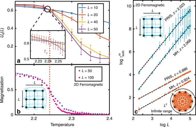
a Binder cumulants U4(L) for various graph sizes L on the 2D Ferromagnetic Ising model. Their intersection determines the critical temperature of the model TC (denoted by a dotted line). b Magnetization estimated from the PRIS for various L. c Scaling of the PRIS magnetization autocorrelation time for various Ising models, benchmarked versus the Metropolis-Hastings algorithm (MH). The complexity of a single time step scales like N2 = L4 for MH on a CPU and like N = L2 for the PRIS on a photonic platform. For readability, error bars in b are not shown (see Supplementary Note 4).

Full size image

In Fig. 4c, we benchmark the performance of the PRIS against the well-known Metropolis-Hastings (MH) algorithm1,68,69. In the context of heuristic methods, one should compare the autocorrelation time of a given observable. The scaling of the magnetization autocorrelation time \({\tau }_{{\rm{auto}}}^{m}={\mathcal{O}}({L}^{z})={\mathcal{O}}({N}^{z/2})\) at the critical temperature is shown in Fig. 4c for two analytically-solvable models: the two-dimensional ferromagnetic and the infinite-range Ising models. Both algorithms yield autocorrelation time critical exponents close to the theoretical value (z ~ 2.1)1 for the two-dimensional Ising model. However, the PRIS seems to perform better on denser models such as the infinite-range Ising model, where it yields a smaller autocorrelation time critical exponent. More significantly, the advantage of the PRIS resides in its possible implementation with any matrix-to-vector accelerator, such as parallel photonic networks, so that the computational (time) complexity of a single step is \({\mathcal{O}}(N)\)34,38,39. Thus, the computational complexity of generating an uncorrelated sample scales like \({\mathcal{O}}({N}^{1+{z}_{{\rm{PRIS}}}/2})\) for the PRIS on a parallel architecture, while it scales like \({\mathcal{O}}({N}^{2+{z}_{{\rm{MH}}}/2})\) for a sequential implementation of MH, on a CPU for instance. Implementing the PRIS on a photonic parallel architecture also ensures that the prefactor in this order of magnitude estimate is small (and only limited by the clock rate of a single recurrent step of this high-speed network). Thus, as long as zPRIS < zMH + 2, the PRIS exhibits a clear advantage over MH implemented on a sequential architecture.