Testing the equality of coefficients – Same Independent, Different Dependent variables

As promised earlier, here is one example of testing coefficient equalities in SPSS, Stata, and R.

Here we have different dependent variables, but the same independent variables. This is taken from Dallas survey data (original data link, survey instrument link), and they asked about fear of crime, and split up the questions between fear of property victimization and violent victimization. Here I want to see if the effect of income is the same between the two. People in more poverty tend to be at higher risk of victimization, but you may also expect people with fewer items to steal to be less worried. Here I also control for the race and the age of the respondent.

The dataset has missing data, so I illustrate how to select out for complete case analysis, then I estimate the model. The fear of crime variables are coded as Likert items with a scale of 1-5, (higher values are more safe) but I predict them using linear regression (see the Stata code at the end though for combining ordinal logistic equations using suest). Race is of course nominal, and income and age are binned as well, but I treat the income bins as a linear effect. I pasted the codebook for all of the items at the end of the post.

These models with multiple dependent variables have different names, economists call them seemingly unrelated regression, psychologists will often just call them multivariate models, those familiar with structural equation modeling can get the same results by allowing residual covariances between the two outcomes — they will all result in the same coefficient estimates in the end.

In SPSS we can use the GLM procedure to estimate the model. Simultaneously we can specify particular contrasts to test whether the income coefficient is different for the two outcomes.

*Grab the online data.
SPSSINC GETURI DATA URI="https://dl.dropbox.com/s/r98nnidl5rnq5ni/MissingData_DallasSurv16.sav?dl=0" FILETYPE=SAV DATASET=MissData.

*Conducting complete case analysis.
COUNT MisComplete = Safety_Violent Safety_Prop Gender Race Income Age (MISSING).
COMPUTE CompleteCase = (MisComplete = 0).
FILTER BY CompleteCase.


*This treats the different income categories as a continuous variable.
*Can use GLM to estimate seemingly unrelated regression in SPSS and test.
*equality of the two coefficients.
GLM Safety_Violent Safety_Prop BY Race Age WITH Income
  /DESIGN=Income Race Age
  /PRINT PARAMETER
  /LMATRIX Income 1
  /MMATRIX ALL 1 -1.

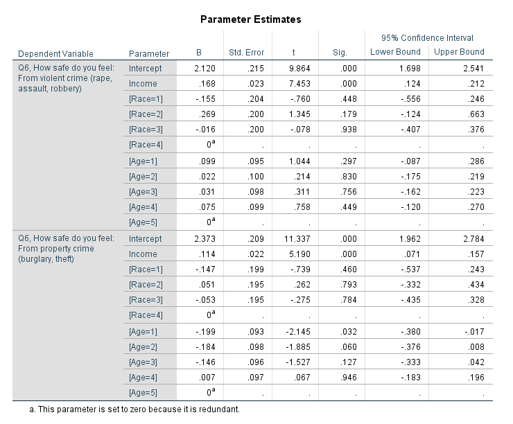
FILTER OFF.  

In the output you can see the coefficient estimates for the two equations. The income effect for violent crime is 0.168 (0.023) and for property crime is 0.114 (0.022).

And then you get a separate table for the contrast estimates.

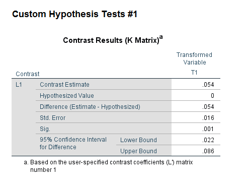
You can see that the contrast estimate, 0.054, equals 0.168 – 0.114. The standard error in this output (0.016) takes into account the covariance between the two estimates. Here you would reject the null that the effects are equal across the two equations, and the effect of income is larger for violent crime. Because higher values on these Likert scales mean a person feels more safe, this is evidence that those with higher incomes are more likely to be fearful of property victimization, controlling for age and race.

Unfortunately the different matrix contrasts are not available in all the different types of regression models in SPSS. You may ask whether you can fit two separate regressions and do this same test. The answer is you can, but that makes assumptions about how the two models are independent — it is typically more efficient to estimate them at once, and here it allows you to have the software handle the Wald test instead of constructing it yourself.

As I stated previously, seemingly unrelated regression is another name for these multivariate models. So we can use the R libraries systemfit to estimate our seemingly unrelated regression model, and then use the library multcomp to test the coefficient contrast. This does not result in the exact same coefficients as SPSS, but devilishly close. You can download the csv file of the data here.

library(systemfit) #for seemingly unrelated regression
library(multcomp)  #for hypothesis tests of models coefficients

#read in CSV file
SurvData <- read.csv(file="MissingData_DallasSurvey.csv",header=TRUE)
names(SurvData)[1] <- "Safety_Violent" #name gets messed up because of BOM

#Need to recode the missing values in R, use NA
NineMis <- c("Safety_Violent","Safety_Prop","Race","Income","Age")
#summary(SurvData[,NineMis])
for (i in NineMis){
  SurvData[SurvData[,i]==9,i] <- NA
}

#Making a complete case dataset
SurvComplete <- SurvData[complete.cases(SurvData),NineMis]
#Now changing race and age to factor variables, keep income as linear
SurvComplete$Race <- factor(SurvComplete$Race, levels=c(1,2,3,4), labels=c("Black","White","Hispanic","Other"))
SurvComplete$Age <- factor(SurvComplete$Age, levels=1:5, labels=c("18-24","25-34","35-44","45-54","55+"))
summary(SurvComplete)

#now fitting seemingly unrelated regression
viol <- Safety_Violent ~ Income + Race + Age
prop <- Safety_Prop ~ Income + Race + Age
fitsur <- systemfit(list(violreg = viol, propreg= prop), data=SurvComplete, method="SUR")
summary(fitsur)

#testing whether income effect is equivalent for both models
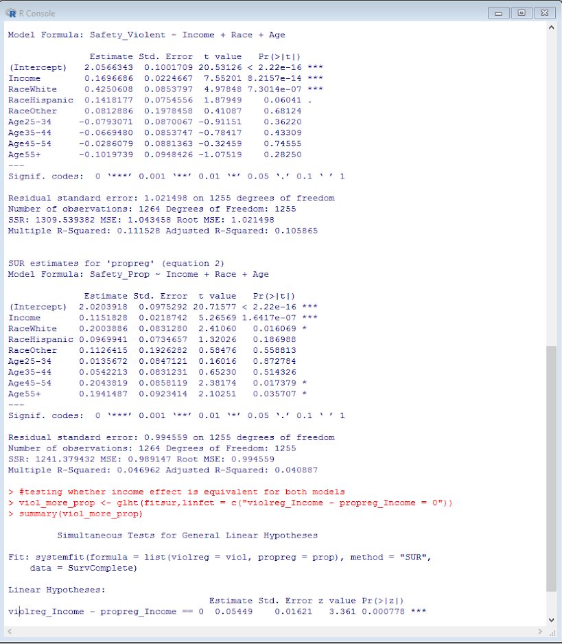
viol_more_prop <- glht(fitsur,linfct = c("violreg_Income - propreg_Income = 0"))
summary(viol_more_prop) 

Here is a screenshot of the results then:

This is also the same as estimating a structural equation model in which the residuals for the two regressions are allowed to covary. We can do that in R with the lavaan library.

library(lavaan)

#for this need to convert factors into dummy variables for lavaan
DumVars <- data.frame(model.matrix(~Race+Age-1,data=SurvComplete))
names(DumVars) <- c("Black","White","Hispanic","Other","Age2","Age3","Age4","Age5")

SurvComplete <- cbind(SurvComplete,DumVars)

model <- '
    #regressions
     Safety_Prop    ~ Income + Black + Hispanic + Other + Age2 + Age3 + Age4 + Age5
     Safety_Violent ~ Income + Black + Hispanic + Other + Age2 + Age3 + Age4 + Age5
    #residual covariances
     Safety_Violent ~~ Safety_Prop
     Safety_Violent ~~ Safety_Violent
     Safety_Prop ~~ Safety_Prop
'

fit <- sem(model, data=SurvComplete)
summary(fit)

I’m not sure offhand though if there is an easy way to test the coefficient differences with a lavaan object, but we can do it manually by grabbing the variance and the covariances. You can then see that the differences and the standard errors are equal to the prior output provided by the glht function in multcomp.

#Grab the coefficients I want, and test the difference
PCov <- inspect(fit,what="vcov")
PEst <- inspect(fit,what="list")
Diff <- PEst[9,'est'] - PEst[1,'est']
SE <- sqrt( PEst[1,'se']^2 + PEst[9,'se']^2 - 2*PCov[9,1] )
Diff;SE

Stata

In Stata we can replicate the same prior analyses. Here is some code to simply replicate the prior results, using Stata’s postestimation commands (additional examples using postestimation commands here). Again you can download the csv file used here. The results here are exactly the same as the R results.

*Load in the csv file
import delimited MissingData_DallasSurvey.csv, clear

*BOM problem again
rename ïsafety_violent safety_violent

*we need to specify the missing data fields.
*for Stata, set missing data to ".", not the named missing value types.
foreach i of varlist safety_violent-ownhome {
    tab `i'
}

*dont specify district
mvdecode safety_violent-race income-age ownhome, mv(9=.)
mvdecode yearsdallas, mv(999=.)

*making a variable to identify the number of missing observations
egen miscomplete = rmiss(safety_violent safety_prop race income age)
tab miscomplete
*even though any individual question is small, in total it is around 20% of the cases

*lets conduct a complete case analysis
preserve 
keep if miscomplete==0

*Now can estimate multivariate regression, same as GLM in SPSS
mvreg safety_violent safety_prop = income i.race i.age

*test income coefficient is equal across the two equations
lincom _b[safety_violent:income] - _b[safety_prop:income]

*same results as seemingly unrelated regression
sureg (safety_violent income i.race i.age)(safety_prop income i.race i.age)

*To use lincom it is the exact same code as with mvreg
lincom _b[safety_violent:income] - _b[safety_prop:income]

*with sem model
tabulate race, generate(r)
tabulate age, generate(a)
sem (safety_violent <- income r2 r3 r4 a2 a3 a4 a5)(safety_prop <- income r2 r3 r4 a2 a3 a4 a5), cov(e.safety_violent*e.safety_prop) 

*can use the same as mvreg and sureg
lincom _b[safety_violent:income] - _b[safety_prop:income]

You will notice here it is the exact some post-estimation lincom command to test the coefficient equality across all three models. (Stata makes this the easiest of the three programs IMO.)

Stata also allows us to estimate seemingly unrelated regressions combining different generalized outcomes. Here I treat the outcome as ordinal, and then combine the models using seemingly unrelated regression.

*Combining generalized linear models with suest
ologit safety_violent income i.race i.age
est store viol

ologit safety_prop income i.race i.age
est store prop

suest viol prop

*lincom again!
lincom _b[viol_safety_violent:income] - _b[prop_safety_prop:income]

An application in spatial criminology is when you are estimating the effect of something on different crime types. If you are predicting the number of crimes in a spatial area, you might separate Poisson regression models for assaults and robberies — this is one way to estimate the models jointly. Cory Haberman and Jerry Ratcliffe have an application of this as well estimate the effect of different crime types at different times of day – e.g. the effect of bars in the afternoon versus the effect of bars at nighttime.

Codebook

Here is the codebook for each of the variables in the database.

Safety_Violent  
    1   Very Unsafe
    2   Unsafe
    3   Neither Safe or Unsafe
    4   Safe
    5   Very Safe
    9   Do not know or Missing
Safety_Prop 
    1   Very Unsafe
    2   Unsafe
    3   Neither Safe or Unsafe
    4   Safe
    5   Very Safe
    9   Do not know or Missing
Gender  
    1   Male
    2   Female
    9   Missing
Race    
    1   Black
    2   White
    3   Hispanic
    4   Other
    9   Missing
Income  
    1   Less than 25k
    2   25k to 50k
    3   50k to 75k
    4   75k to 100k
    5   over 100k
    9   Missing
Edu 
    1   Less than High School
    2   High School
    3   Some above High School
    9   Missing
Age 
    1   18-24
    2   25-34
    3   35-44
    4   45-54
    5   55+
    9   Missing
OwnHome 
    1   Own
    2   Rent
    9   Missing
YearsDallas
    999 Missing