
8

【statsmodels】OLS最小二乘法
source link: https://www.guofei.site/2019/03/03/statsmodels_ols.html
Go to the source link to view the article. You can view the picture content, updated content and better typesetting reading experience. If the link is broken, please click the button below to view the snapshot at that time.

【statsmodels】OLS最小二乘法
2019年03月03日Author: Guofei
文章归类: 4-1-统计模型 ,文章编号: 409
版权声明:本文作者是郭飞。转载随意,但需要标明原文链接,并通知本人
原文链接:https://www.guofei.site/2019/03/03/statsmodels_ols.html
几种回归模型概述
介绍一下几种与回归statistical model1有关的模型
Y=Xβ+uY=Xβ+u,where u∼N(0,Σ)u∼N(0,Σ)
- OLS : ordinary least squares for i.i.d. errors :Σ=IΣ=I
- WLS : weighted least squares for heteroskedastic errors :diag(Σ)diag(Σ)
- GLS : generalized least squares for arbitrary covariance :ΣΣ
- GLSAR : feasible generalized least squares with autocorrelated AR(p) errors :Σ=Σ(ρ)Σ=Σ(ρ)
OLS
setp1. 载入包和数据
import numpy as np
import matplotlib.pyplot as plt
import pandas as pd
import statsmodels.formula.api as smf

df = pd.DataFrame()
df.loc[:, 'x'] = np.linspace(start=0, stop=20, num=50)
df.loc[:, 'y'] = 2 * df.x + np.random.randn(50) + 5
step2. 构建模型
lm_s = smf.ols(formula='y ~ x', data=df).fit()
step3. 预测
from statsmodels.sandbox.regression.predstd import wls_prediction_std
prstd, iv_l, iv_u = wls_prediction_std(lm_s)
#     predstd : standard error of prediction
#     interval_l, interval_u : lower und upper confidence bounds
fig, ax = plt.subplots(figsize=(8, 6))
ax.plot(df.x, df.y, 'o', label="data") # 输入样本
ax.plot(df.x, lm_s.predict(df), 'r--.', label="OLS") # 预测值
ax.plot(df.x, iv_u, 'r--') # 预测上界
ax.plot(df.x, iv_l, 'r--') # 预测下界
ax.legend(loc='best')
plt.show()
step4. 模型结果
lm_s.predict(df) # 返回预测值y,是一个array
lm_s.resid # 返回残差,是一个pd.Series
lm_s.params # 返回参数估计值,是pd.Series类型

lm_s.summary()
lm_s.rsquared #R^2
lm_s.rsquared_adj

lm_s.aic # 越低越好
lm_s.bic # 越低越好
step5. 残差分析
sm.stats.linear_rainbow(lm_s)
sm.stats.durbin_watson(lm_s.resid) #dw检验
官网上还有多种检验方法 http://www.statsmodels.org/stable/stats.html#residual-diagnostics-and-specification-tests
除此之外还有一些不常用的属性,例如自由度、似然值等等,就不摘抄了,看官网
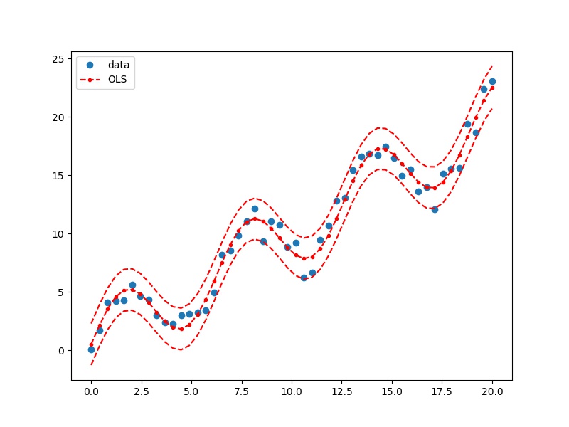
用ols做非线性回归
官网是用OLS对象做的,这里用formula重做一遍
import numpy as np
import matplotlib.pyplot as plt
import pandas as pd
import statsmodels.formula.api as smf

df = pd.DataFrame()
df.loc[:, 'x'] = np.linspace(start=0, stop=20, num=50)
df.loc[:, 'y'] = np.sin(df.x) * 3 + df.x + np.random.randn(50)

# %%
lm_s = smf.ols(formula='y ~ np.sin(x)+x', data=df).fit()

# %%

from statsmodels.sandbox.regression.predstd import wls_prediction_std

prstd, iv_l, iv_u = wls_prediction_std(lm_s)
#     predstd : standard error of prediction
#     interval_l, interval_u : lower und upper confidence bounds
fig, ax = plt.subplots(figsize=(8, 6))
ax.plot(df.x, df.y, 'o', label="data")
ax.plot(df.x, lm_s.predict(df), 'r--.', label="OLS")
ax.plot(df.x, iv_u, 'r--')
ax.plot(df.x, iv_l, 'r--')
ax.legend(loc='best')
plt.show()
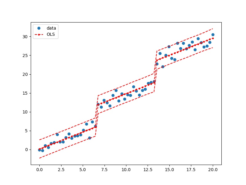
用ols做哑变量回归
import numpy as np
import matplotlib.pyplot as plt
import pandas as pd
import statsmodels.formula.api as smf

df = pd.DataFrame()
df.loc[:, 'x1'] = np.linspace(start=0, stop=20, num=60)
df.loc[:,'x2']=[0]*20+[1]*20+[2]*20
df.loc[:, 'y'] = df.x1 + 5*df.x2+np.random.randn(60)

# %%
lm_s = smf.ols(formula='y ~ np.sin(x1)+x1+x2', data=df).fit()

# %%

from statsmodels.sandbox.regression.predstd import wls_prediction_std

prstd, iv_l, iv_u = wls_prediction_std(lm_s)
#     predstd : standard error of prediction
#     interval_l, interval_u : lower und upper confidence bounds
fig, ax = plt.subplots(figsize=(8, 6))
ax.plot(df.x1, df.y, 'o', label="data")
ax.plot(df.x1, lm_s.predict(df), 'r--.', label="OLS")
ax.plot(df.x1, iv_u, 'r--')
ax.plot(df.x1, iv_l, 'r--')
ax.legend(loc='best')
plt.show()
OLS的结果检验
- F检验,用来检验方程的显著性
lm_s.f_test('x1=x2=0') - 多重共线性
lm_s.summary()
# Cond. No. 这一项太大的话,可能有多重共线性。也会在warning中列出
ridge
ols('y~x1+x2',data=df).fit_regularized(alpha=1, L1_wt=1)
TODO:LASSO, ElasticNet
R-style formulas
import statsmodels.api as sm
import statsmodels.formula.api as smf
df = sm.datasets.get_rdataset("Guerry", "HistData").data
df = df[['Lottery', 'Literacy', 'Wealth', 'Region']].dropna()
Categorical variables
res = smf.ols(formula='Lottery ~ Literacy + Wealth + Region', data=df).fit()

# C指的是Categorical variables
res = smf.ols(formula='Lottery ~ Literacy + Wealth + C(Region)', data=df).fit()
-1
# -1 指的是使 Intercept = 0
res = smf.ols(formula='Lottery ~ Literacy + Wealth + C(Region) -1 ', data=df).fit()
print(res.summary())
冒号和乘号
# “:” adds a new column to the design matrix with the product of the other two columns. “
# *” will also include the individual columns that were multiplied together:
# 所以'Lottery ~ Literacy * Wealth - 1' 相当于 'Lottery ~ Literacy + Wealth+Literacy : Wealth - 1'
res1 = smf.ols(formula='Lottery ~ Literacy : Wealth - 1', data=df).fit()
res2 = smf.ols(formula='Lottery ~ Literacy * Wealth - 1', data=df).fit()
print(res1.params)
print(res2.params)
Functions
- 直接使用numpy
res = smf.ols(formula='Lottery ~ np.log(Literacy)', data=df).fit() - 使用自定义函数
def plus_1(x):
 return x+1.0
res = smf.ols(formula='Lottery ~ plus_1(Literacy)', data=df).fit()
参考资料
您的支持将鼓励我继续创作!
Recommend
About Joyk
Aggregate valuable and interesting links.
Joyk means Joy of geeK