Longest Job First (LJF) CPU scheduling algorithm

Prerequisite – Process Management | CPU Scheduling
Longest Job First (LJP) is a non-preemptive scheduling algorithm. This algorithm is based upon the burst time of the processes. The processes are put into the ready queue based on their burst times i.e., in a descending order of the burst times. As the name suggests this algorithm is based upon the fact that the process with the largest burst time is processed first. The burst time of only those processes is considered that have arrived in the system until that time. Its preemptive version is called Longest Remaining Time First (LRTF) algorithm.

Procedure:

• Step-1:
  First, sort the processes in increasing order of their Arrival Time.
• Step-2:
  Choose the process having highest Burst Time among all the processes that have arrived till that time. Then process it for its burst time. Check if any other process arrives until this process completes execution.
• Step-3:
  Repeat the above both steps until all the processes are executed.

Note-
If two processes have the same burst time then the tie is broken using FCFS i.e., the process that arrived first is processed first.
Disadvantages-

• This algorithm gives very high average waiting time and average turn-around time for a given set of processes.
• This may lead to convoy effect.
• It may happen that a short process may never get executed and the system keeps on executing the longer processes.
• It reduces the processing speed and thus reduces the efficiency and utilization of the system.

Let us consider the following examples.

Example-1: Consider the following table of arrival time and burst time for four processes P1, P2, P3 and P4.

Process   Arrival time   Burst Time
P1            1 ms          2 ms
P2            2 ms          4 ms
P3            3 ms          6 ms
P4            4 ms          8 ms  

Working:

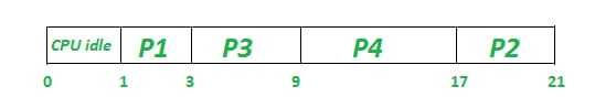
1. At t = 1, Available Process : P1. So, select P1 and execute 2 ms.
2. At t = 3 i.e. after P1 gets executed, Available Process : P2, P3. So, select P3 and execute 6 ms (since BT(P3)=6 which is higher than BT(P2) = 4)
3. At t = 9 i.e. after execution of P3, Available Process : P2, P4. So, select P4 and execute 8 ms (since, BT(P4) = 8, BT(P2) = 4)
4. Finally execute the process P2 for 4 ms.

Note –
CPU will be idle for 0 to 1 unit time since there is no process available in the given interval.

Gantt chart will be as following below,

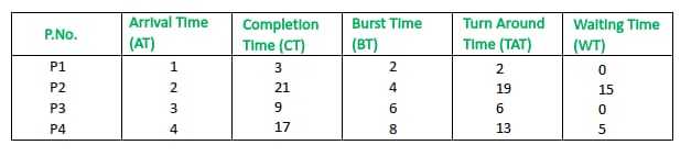
Since, complietion time (CT) can be directly determined by Gantt chart, and

Turn Around Time (TAT)
= (Completion Time) - (Arival Time)

Also, Waiting Time (WT)
= (Turn Around Time) - (Burst Time) 

Therefore, final table look like,

Output :

Total Turn Around Time = 40 ms
So, Average Turn Around Time = 40/4 = 10.00 ms

And, Total Waiting Time = 20 ms
So Average Waiting Time = 20/4 = 5.00 ms 

Example-2: Consider the following table of arrival time and burst time for four processes P1, P2, P3, P4 and P5.

Process   Arrival time   Burst Time
P1            0 ms          2 ms
P2            0 ms          3 ms
P3            2 ms          2 ms
P4            3 ms          5 ms 
P5            4 ms          4 ms 

Working :
Gantt chart for this example,

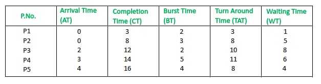
Since, complietion time (CT) can be directly determined by Gantt chart, and

Turn Around Time (TAT)
= (Completion Time) - (Arival Time)

Also, Waiting Time (WT)
= (Turn Around Time) - (Burst Time) 

Therefore, final table look like,

Output :

Total Turn Around Time = 40 ms
So, Average Turn Around Time = 40/5 = 8 ms

And, Total Waiting Time = 24 ms
So, Average Waiting Time = 24/5 = 4.8 ms 

Attention reader! Don’t stop learning now. Get hold of all the important CS Theory concepts for SDE interviews with the CS Theory Course at a student-friendly price and become industry ready.