Using Perlin Noise to Generate 2D Terrain and Water

This post is going to be the Perlin noise tutorial that I've always wanted to see. By the end of it, we'll procedurally generate 2D terrain and water with GLSL.

Why Another Perlin Noise Write-Up?

Perlin noise was invented in the eighties and has since been used countless times to generate natural-looking visual effects in films and games.

If you google "perlin noise", you will get a trove of articles and code. However, in my opinion, a beginner will have a hard time figuring out how it really works. I think that a lot of articles on the subject don't provide enough context, jump into too much detail too quickly and use scary terminology like "surflets". I've even stumbled upon some articles presenting blurred white noise as perlin noise, which is not the case!

And that's why I decided to try and write a more beginner-friendly article on the subject, that starts from a simple and easy to understand case, and builds up towards a more advanced one. Hopefully, people who read this tutorial won't have to struggle any more!

Noise Is a Function

Before we go any further, I want to make sure a simple, but very important point is understood: noise is a mathematical function, just like the sine or the exponent. The gray, amorphous, lumpy fog that you see in most pictures is just one of the possible graphical representations of said function. The reason I want to make this explicit is that some people may think about calculating noise in terms of pixels being affected by neighbor pixels, which really isn't the correct way to think about Perlin noise.

Most of us are familiar with mathematical functions of a single variable (again, sine for example), but functions can depend on multiple variables. It's fairly easy to visually represent a function of two variables. For a function of three variables, you can imagine the time, t, as the third variable, and the graphical representation would be animated: the values of the function along the z at each point (x, y) would change with the passage of time.

Now, if you image-search for perlin noise, what you'll usually see is the graphical representation of a two-dimensional function, where lighter pixels correspond to higher values at particular x and y coordinates. But the thing is, perlin noise doesn't have to be two-dimensional. The concept can be extended to any number of dimensions. But more importantly for us, it can be reduced to just a single dimension! And, for us mere mortals, it's much easier to understand how the one-dimensional case works. Armed with that knowledge, we'll be ready to tackle the more complex cases. That is the approach that this post is going to take.

Requirements for the Noise Function

Regardless of dimensionality, the noise function must be continuous, smooth and random-looking. Of course, there are strict mathematical definitions for what things like "continuous" and "smooth" mean, but you needn't worry about that right now - just go with your intuitive understanding.

In the one-dimensional case, the graph of a function possessing the above-mentioned properties will look like a neat squiggly line. Our first goal will be to construct such a function.

It should be noted that there are multiple methods to construct a function fitting these criteria, Perlin's technique is just one of them.

Constructing the Noise Function of One Variable

As promised, we're going to consider the single-variable case first. Thus, our noise function n is defined in the domain of real numbers, R.

Now, let's imagine that for each integer, a value of either 1 or -1 is chosen randomly. For a given integer i, we're going to denote the corresponding randomly chosen value as g(i). We'll call these values gradients.

The noise function is defined as follows:

n(p) = (1 - F(p-p0))g(p0)(p-p0) + F(p-p0)g(p1)(p-p1)

Where:

• p0 = floor(p) (largest integer smaller than or equal to p)
• p1 = p0 + 1 (smallest integer larger than p)
• g(p0) and g(p1) are the gradients at p0 and p1 respectively
• F(t) = t3(t(t-15)+10), a fade function, the purpose of which will be explained a bit later

As you can see, it's just interpolating between two values, g(p0)(p-p0) and g(p1)(p-p1), with the interpolation parameter given by applying the fade function to p-p0. The noise function turns out to have a number of interesting properties (the rigorous proof of which isn't within the scope of the article):

• The values of this function at integer points are zero (this property is actually easy to see)
• The value of the function will decrease as its argument approaches an integer for which -1 was randomly chosen as the gradient value.
• Conversely, the value of the function will increase as its argument approaches an integer for which 1 was chosen as the gradient value.
• The function is continuous and smooth

Explained in a handwavy kind of way, the technique boils down to randomly specifying the desired kind of growth (positive or negative) in the neighborhood of each integer point of the function's domain and then fitting a nice smooth curve that satisfies the growth requirements, with the caveat that the function's values must be 0 at integer points.

Of course, showing is better than telling, so I suggest you play with the following interactive demo to get an intuitive sense of how the function works (javascript must be enabled):

Fade Function Explained

I still owe you an explanation for that "fade function" polynomial. I won't go too deep into it for the sake of brevity, but I'll try to give you an idea.

First, try unchecking the "apply fade function" checkbox in the demo and observe the results. Doesn't look very smooth, does it? Look at these sharp corners!

Without the fade function, our noise becomes constant 0 between integer points with the same gradient values. On the surface, it's easy to see why: if you just plug in the same gradient values for p0 and p1 into the expression for noise without the fade function, it'll be zero. But there's a bit more to it than that, and we'll need just a bit of calculus to explain it.

Before we proceed with the explanation, we need to strictly define what it means for a function to be "smooth". A function is called Ci-smooth if it has continuous derivatives of up to i-th order (in case your calculus is rusty, or these words don't sound familiar at all, I suggest consulting your favorite calculus textbook or Wikipedia).

Now, if you don't apply the fade function to the interpolation parameter and instead use p-p0 directly, the resulting function will not be smooth enough. You can try doing it yourself: replace F(p-p0) with just p-p0 in the noise function definition, simplify the expression and try working out the derivative. The equation for the derivative between p0 and p1 is going to look like (some constant value)*p + (some other constant value), in other words it'll be a straight line. The constants depend on p0 and p1, so the derivative for the overall noise function will look like a bunch of various straight lines. We don't even have a continuous first-order derivative, so our function isn't smooth at all!

Basically, applying the fade gives our noise function continuous higher-order derivatives which makes it look nice and smooth. Instead of varying the interpolation parameter from 0 to 1 linearly, the fade function varies it along an s-shaped curve.

Assigning a Random Value to Each Integer

Before we move on to the implementation, something needs to be mentioned about how we're going to randomly pick gradient values for each integer point of the noise function's domain. The way it's done in the "classic" implementation (and the way you'll most likely encounter in other Perlin noise write-ups) goes something like this:

• An array P of integers from 0 to 256 is permutated at random. Of course, this isn't done at runtime; usually the random permutation is simply hardcoded. Also, it is repeated 2 times in a row, so that Perlin ends up containing 512 elements (this is needed to simplify the next step).
• A value is looked up from P based on the point the gradient of which we're trying to determinine (i.e. for single-dimensional case it will be P[x & 0xff], for 2-dimensional it will be P[P[P[x & 0xff] + (y & 0xff)]], etc.)
• The value from the previous lookup is used to look up into an array of uniformly distributed gradient values

I don't want you to dwell on this too much though, because it is an implementation detail that is not critical to understanding how the overall technique works. Different methods can be used for this. For example, if you're trying to implement Perlin noise in a shader using WebGL, you cannot use the described method because WebGL shaders can't use variable indices with arrays. Instead, you can read the values from a texture filled with random RGB values, and it'll pretty much work the same.

Implementation

Now we've got everything ready to implement one-dimensional perlin noise. I'm going to use GLSL for this, because then I can paste the code into Shadertoy which is very handy for online demos like this. The code should be portable to other languages with minimal changes though.

The fade function is straightforward, so I'm not going to explain it.

float fade(float t) {
  return t*t*t*(t*(t*6.0 - 15.0) + 10.0);
}

Now comes the grad function. It returns a gradient value for a given integer p. We're using WebGL and can't do variable indexes into arrays, so we're going to sample from a random RGB texture and return 1 if the red channel is > 0.5, and -1 otherwise.

float grad(float p) {
  const float texture_width = 256.0;
	float v = texture2D(iChannel0, vec2(p / texture_width, 0.0)).r;
  return v > 0.5 ? 1.0 : -1.0;
}

A few points need to be made that aren't apparent from the code:

• The texture needs to be repeated (i.e. both TEXTURE_WRAP_S and TEXTURE_WRAP_T options need to be set to REPEAT) so that values that are greater than the pixel size of the texture (or even negative values) can be used with texture2D.
• The texture needs to use nearest-neighbor filtering.

Finally, here's the function that computes noise:

float noise(float p) {
  float p0 = floor(p);
  float p1 = p0 + 1.0;
    
  float t = p - p0;
  float fade_t = fade(t);

  float g0 = grad(p0);
  float g1 = grad(p1);
  
  return (1.0-fade_t)*g0*(p - p0) + fade_t*g1*(p - p1);
}

It's pretty self-explanatory and just follows the formula I gave at the start of the article.

Finally, let's take a closer look at the main function of the shader where we actually use the noise function.

void mainImage( out vec4 fragColor, in vec2 fragCoord )
{
    const float frequency = 1.0 / 20.0;
    const float amplitude = 1.0 / 5.0;
    float n = noise(fragCoord.x * frequency) * amplitude;
    float y = 2.0 * (fragCoord.y/iResolution.y) - 1.0; /* map fragCoord.y into [-1; 1] range */
    vec3 color = n >  y ? vec3(1.0) : vec3(0.0);
    fragColor = vec4(color, 1.0);
}

We need the frequency parameter, because without it the samples of the noise function would be too close together and we wouldn't be able to see anything. The amplitude parameter is there simply to control the heights of peaks/troughs. You can play with these parameters yourself to understand how they affect the final look:

Making the Noise Look More Interesting

At this point, we've covered the core of what makes Perlin noise work. Now is the time to apply it to make something interesting-looking. The trick is to sample the noise function multiple times, with different frequencies and amplitudes, and add the results up. That is called "fractal noise".

The bulk of the shader stays the same, the only part that changes is the main function:

void mainImage( out vec4 fragColor, in vec2 fragCoord )
{
    /* Add up noise samples with different frequencies and amplitudes. */
    float n =
        noise(fragCoord.x * (1.0/300.0)) * 1.0 +
        noise(fragCoord.x * (1.0/150.0)) * 0.5 +
        noise(fragCoord.x * (1.0/75.0))  * 0.25 +
        noise(fragCoord.x * (1.0/37.5))  * 0.125;
    float y = 2.0 * (fragCoord.y/iResolution.y) - 1.0; /* map fragCoord.y into [-1; 1] range */
    vec3 color = n >  y ? vec3(0.0) : vec3(1.0);
	fragColor = vec4(color, 1.0);
}

By manipulating frequencies and amplitudes, you can control how the result looks: lower frequencies give you gently sloped hills, while higher frequencies with higher amplitudes give you more jagged, spiky look. Play with the demo yourself:

Intermission: Scrolling 2D Terrain!

Using the stuff covered that we covered so far, it's easy to put together a simple demo that endlessly flies you past a 2d mountain range! The demo below uses the time counter (shadertoy-specific) for scrolling, and it uses different factors for it on the foreground and background mountains to achieve a nice parallax effect.

Jump to the Second Dimension

Hopefully by now you have a solid understanding of the the one-dimensional case. You should be well-equipped then to deal with the two-dimensional case.

At this point I should explain why we call those random values corresponding to integer points "gradients". In mathematics, the term gradient is used to refer to the direction in which a function experiences the fastest growth at a given point. In other words, "gradient at a given point p" answers the question: "from a given point p, which direction should the argument go in order for the function to grow the most?". In case of single-variable functions, the argument can either go forwards (corresponding to gradient value of 1) or backwards (corresponding to gradient value -1). In the case of two-dimensional functions, the gradient has to be a unit 2d vector, because the argument can change in any direction on the XY plane.

So the first thing we should do is modify our grad function to give us a random two-dimensional unit vector:

vec2 grad(vec2 p) {
	const float texture_width = 256.0;
	vec4 v = texture2D(iChannel0, vec2(p.x / texture_width, p.y / texture_width));
    return normalize(v.xy*2.0 - vec2(1.0)); /* remap sampled value to [-1; 1] and normalize */
}

Note that the values sampled from the texture are in the range [0, 1], and it is imperative that we remap them to the [-1, 1] range. If we don't, our gradients won't be random enough (they'll be clustered 1/4th of the range they should be in) and the result will be ugly. Also, notice the call to normalize: it's important to ensure that the gradient is a unit vector.

The noise function requires a little more changes. But first, let's recap what we did to calculate noise at point p in the 1D case:

• We determined the integers p0 and p1 surrounding the point p
• For both p0 and p1, we calculated the product between the gradient at that point, and the difference between p and that point.
• Finally, we did an interpolation between the values calculated in the previous step

When you extend this to two dimensions, you get:

• Determine the four integer points on the plane p0, p1, p2 and p3 surrounding the point p ("lattice points")
• For each of those four lattice points, calculate the dot product between the gradient at the lattice point and the direction from the lattice point to the point p
• Do something similar to bilinear interpolation: interpolate between the dot products corresponding to the top two lattice points, then interpolate between the dot products corresponding to the two bottom lattice points. Finally, interpolate between the results of the previous two interpolations.

So, overall, the idea is pretty much the same as in the 1D case, it's just that scalar values have become 2D vectors!

Here is the code:

/* 2D noise */
float noise(vec2 p) {
  /* Calculate lattice points. */
  vec2 p0 = floor(p);
  vec2 p1 = p0 + vec2(1.0, 0.0);
  vec2 p2 = p0 + vec2(0.0, 1.0);
  vec2 p3 = p0 + vec2(1.0, 1.0);
  
  /* Look up gradients at lattice points. */
  vec2 g0 = grad(p0);
  vec2 g1 = grad(p1);
  vec2 g2 = grad(p2);
  vec2 g3 = grad(p3);
    
  float t0 = p.x - p0.x;
  float fade_t0 = fade(t0); /* Used for interpolation in horizontal direction */

  float t1 = p.y - p0.y;
  float fade_t1 = fade(t1); /* Used for interpolation in vertical direction. */

  /* Calculate dot products and interpolate.*/
  float p0p1 = (1.0 - fade_t0) * dot(g0, (p - p0)) + fade_t0 * dot(g1, (p - p1)); /* between upper two lattice points */
  float p2p3 = (1.0 - fade_t0) * dot(g2, (p - p2)) + fade_t0 * dot(g3, (p - p3)); /* between lower two lattice points */
  
  /* Calculate final result */
  return (1.0 - fade_t1) * p0p1 + fade_t1 * p2p3;
}

Here's how it looks with a few samples of different frequency and amplitude are added together:

2D Water!

If you render 2D noise in the exact same way we did with the 1D noise in the mountains example, but vary the y coordinate with time, you can get a neat effect, resembling rising and falling waves in a body of water. If you also vary the x coordinate with time, you'll get the appearance of rolling waves. You can enhance the effect even further, if you advance the x coordinate for larger, low frequency waves at a slower rate than for smaller, high frequency waves. Check out the demo below:

3D Noise

At this point, you should be able to figure out how to extend the noise function to 3 variables yourself. The only difference now is that the interpolation becomes more involved: the lattice is now three-dimensional, so there are now 8 integer points surrounding the point p. You do the same interpolation as in the 2D case twice: once for the top 4 vertices, once for the bottom 4 vertices, and finally you interpolate between those two results.

Here is the modified version of the noise function.

float noise(vec3 p) {
  /* Calculate lattice points. */
  vec3 p0 = floor(p);
  vec3 p1 = p0 + vec3(1.0, 0.0, 0.0);
  vec3 p2 = p0 + vec3(0.0, 1.0, 0.0);
  vec3 p3 = p0 + vec3(1.0, 1.0, 0.0);
  vec3 p4 = p0 + vec3(0.0, 0.0, 1.0);
  vec3 p5 = p4 + vec3(1.0, 0.0, 0.0);
  vec3 p6 = p4 + vec3(0.0, 1.0, 0.0);
  vec3 p7 = p4 + vec3(1.0, 1.0, 0.0);
    
  /* Look up gradients at lattice points. */
  vec3 g0 = grad(p0);
  vec3 g1 = grad(p1);
  vec3 g2 = grad(p2);
  vec3 g3 = grad(p3);
  vec3 g4 = grad(p4);
  vec3 g5 = grad(p5);
  vec3 g6 = grad(p6);
  vec3 g7 = grad(p7);
    
  float t0 = p.x - p0.x;
  float fade_t0 = fade(t0);

  float t1 = p.y - p0.y;
  float fade_t1 = fade(t1);
    
  float t2 = p.z - p0.z;
  float fade_t2 = fade(t2);

  float p0p1 = (1.0 - fade_t0) * dot(g0, (p - p0)) + fade_t0 * dot(g1, (p - p1));
  float p2p3 = (1.0 - fade_t0) * dot(g2, (p - p2)) + fade_t0 * dot(g3, (p - p3));

  float p4p5 = (1.0 - fade_t0) * dot(g4, (p - p4)) + fade_t0 * dot(g5, (p - p5));
  float p6p7 = (1.0 - fade_t0) * dot(g6, (p - p6)) + fade_t0 * dot(g7, (p - p7));

  float y1 = (1.0 - fade_t1) * p0p1 + fade_t1 * p2p3;
  float y2 = (1.0 - fade_t1) * p4p5 + fade_t1 * p6p7;

  return (1.0 - fade_t2) * y1 + fade_t2 * y2;
}

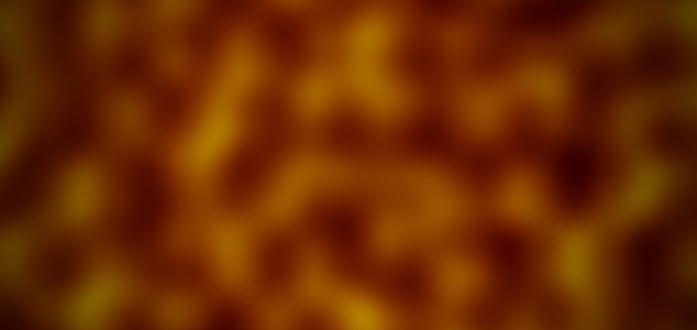
Similarly to what we did in the 2D case, we can move a 2D slice through the 3D noise by varying the third argument with the time counter and get an animated image. With some coloring we can get an effect reselmbling lava or maybe the surface of a glowing star. Demo:

That's It!

Now you too can use perlin noise for your game, demo or whatever it is you're making! The code should be fairly easy to adapt to your language of choice. If you have questions or found something incorrect, let me know in the comments.

---

Like this post? Follow this blog on Twitter for more!