Numerical Methods with C++ Part 1: Newton-Cotes Integration

Welcome to a new post on thoughts-on-cpp.com. This time I would like to start a new series, Numerical Methods. But don’t be disappointed if you’re expecting a new post on the n-body-problem, I’m still planning to continue the “My God, It’s Full of Stars” series. With this new series, I would like to talk about numerical methods which are important in my daily business, starting from Trapezoidal and Simpson integration methods of type Newton-Cotes.

The Newton-Cotes formula is a quadratic numerical approximation for integral calculations. The idea is to interpolate the function, which shall be integrated, by a polynomial with equidistant nodes. The polynomial can be of, for example, a form of aligned trapezoids or aligned parables. Common Newton-Cotes integration polynomial rules are

Trapezoid rule
Simpson rule
Romberg
Pulcherrima
Milne/Boole rule
6-Node rule
Weddle rule

With this post, we will have a closer look at the first two integration rules, Trapezoidal and Simpson.

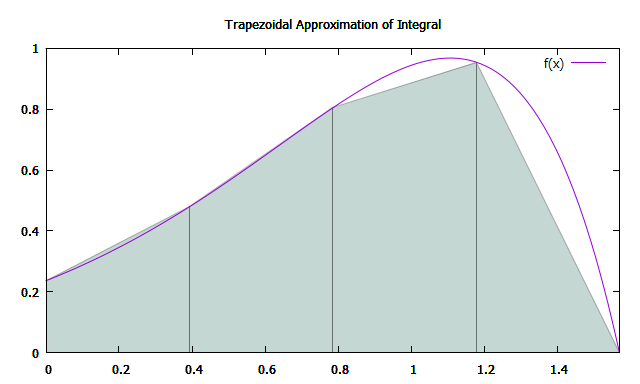
Trapezoidal Integral Approximation

The integral approximation by trapezoids is very simple to explain. All we need to do is to subdivide the example function

$I=\int_0^{\pi/2} \frac{5}{e^\pi-2}\exp(2x)\cos(x)dx=1.0$

we want to integrate into equidistant areas whose exact integrations we can sum up. Clearly, the accuracy of the approximation is depending on the number of subdivisions N. The width of each area is therefore defined by

$\Delta x = \frac{b-a}{N}$

with $a=0$ and $b=\pi/2$ .

Approximation of integral of f(x) between 0 and pi/2 by trapezoids

The area of each trapezoid can be calculated by

$A=\frac{a+b}{2}\cdot h$

and therefore the approximated integral $\widetilde{ I }$ of our function f(x) can be defined as

$\widetilde{ I } = \sum_{i=1}^{N+1} \frac{x_i-x_{i+1}}{2}(f(x_i)+f(x_{i+1}))$

The implementation of the Trapezoidal integration is taking 4 parameters, the range [a,b] of integration of the function f(x), the number of subdivisions n, and the function f(x).

double trapezoidalIntegral(double a, double b, int n, const std::function<double (double)> &f) { const double width = (b-a)/n;

double trapezoidal_integral = 0; for(int step = 0; step < n; step++) { const double x1 = a + step*width; const double x2 = a + (step+1)*width;

trapezoidal_integral += 0.5*(x2-x1)*(f(x1) + f(x2)); }

return trapezoidal_integral; }

Simpson Integral Approximation

The Simpson rule is approximating the integral of the function f(x) by the exact integration of a parable p(x) with nodes at a, b, and $m=\frac{a+b}{2}$ . In order to increase the approximation accuracy, the function can be subdivided by N, similar to the Trapezoidal integral approximation.

Approximation of integral of f(x) between 0 and pi/2 by parabola

Approximation of integral of f(x) between 0 and pi/2 by a parabola

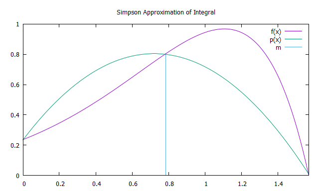
The exact integration can be done by summing up the area of 6 rectangles with equidistant width. The height of the first rectangle is defined by $f(x_a)$ , the height of the next 4 rectangles is defined by $f(\frac{a+b}{2})$ , and the height of the last rectangle is defined by $f(x_b)$ . As a result, the formula of the approximated integral according to Simpson rule can be defined as

$\widetilde{ I } = \sum_{i=1}^{N+1} \frac{x_i-x_{i+1}}{6}(f(x_i)+4f(\frac{a+b}{2})+f(x_{i+1}))$

The implementation of the Simpson integration is, similar to the Trapezoidal based solution, taking 4 parameters, the range [a,b] of integration of the function f(x), the number of subdivisions n, and the function f(x)

double simpsonIntegral(double a, double b, int n, const std::function<double (double)> &f) { const double width = (b-a)/n;

double simpson_integral = 0; for(int step = 0; step < n; step++) { const double x1 = a + step*width; const double x2 = a + (step+1)*width;

simpson_integral += (x2-x1)/6.0*(f(x1) + 4.0*f(0.5*(x1+x2)) + f(x2)); }

return simpson_integral; }

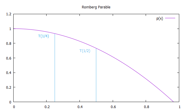
Romberg Integral Approximation

If we integrate the function f(x) with the Trapezoidal approach but bisecting the step size based on the step size of the previous step, we get the approximation sequence

$T(1)=0.18755, \> T(\frac{1}{2})=0.724727, \> T(\frac{1}{4})=0.925565$

The idea of the Romberg integration is now to introduce a y-axis symmetric parable which is crossing the points $T(1), \> T(\frac{1}{2})$ and extrapolate to $x \rightarrow 0$ .

Romberg parable with nodes at T(1/2) and T(1/4)

Therefore every term of the first column R(n,0) of the Romberg integration is equivalent to the Trapezoidal integration, were every solution of the second column R(n,1) is equivalent to the Simpson rule, and every solution of the third column R(n,2) is equivalent to Boole’s rule. As a result, the Formulas for the Romberg integration are

$R(0,0)=h_{1}(f(a)+f(b))$

$R(n, 0)=\frac{1}{2} R(n-1,0)+h_{n} \sum_{k=1}^{2^{\pi-1}} f\left(a+(2 k-1) h_{n}\right)$

$R(n, m)=R(n, m-1)+\frac{R(n, m-1)-R(n-1, m-1)}{4^{m}-1}$

std::vector<std::vector<double>> rombergIntegral(double a, double b, size_t n, const std::function<double (double)> &f) { std::vector<std::vector<double>> romberg_integral(n, std::vector<double>(n));

//R(0,0) Start with trapezoidal integration with N = 1 romberg_integral.front().front() = trapezoidalIntegral(a, b, 1, f);

double h = b-a; for(size_t step = 1; step < n; step++) { h *= 0.5;

//R(step, 0) Improve trapezoidal integration with decreasing h double trapezoidal_integration = 0; size_t stepEnd = pow(2, step – 1); for(size_t tzStep = 1; tzStep <= stepEnd; tzStep++) { const double deltaX = (2*tzStep – 1)*h; trapezoidal_integration += f(a + deltaX); } romberg_integral[step].front() = 0.5*romberg_integral[step – 1].front() + trapezoidal_integration*h;

//R(m,n) Romberg integration with R(m,1) -> Simpson rule, R(m,2) -> Boole's rule for(size_t rbStep = 1; rbStep <= step; rbStep++) { const double k = pow(4, rbStep); romberg_integral[step][rbStep] = (k*romberg_integral[step][rbStep-1] – romberg_integral[step-1][rbStep-1])/(k-1); } }

return romberg_integral; }

The repository numericalIntegration can be found at GitHub. It will also contain the other numerical integration methods, as the name suggests, later on.

Did you like the post?

What are your thoughts?

Feel free to comment and share this post.

Please also join my mailing list, seldom mails, no spam and no advertising, guaranteed.
By clicking submit, you agree to share your email address with the site owner and Mailchimp to receive updates, and other emails from the site owner. Use the unsubscribe link in those emails to opt out at any time.

Numerical Methods with C++ Part 1: Newton-Cotes Integration

Numerical Methods with C++ Part 1: Newton-Cotes Integration

Trapezoidal Integral Approximation

Simpson Integral Approximation

Romberg Integral Approximation

Recommend

Navigator Dot CPU Class

Making WPTouch compatible with Firefox OS

isMobileDevice and the death of innocence [SPOILERS]

What’s A Human-Powered Computer?

笔记本电脑的正确使用方法

user-scalable=like, whatever

(Mobile) Web Compatibility on the World Wide Web

Numerical Methods with C++ Part 2: Gauss-Legendre Integration

Background Positions X and Y. (And ehow.com).

什么是数据分析/数据科学？

About Joyk