A Deep Dive into Lane Detection with Hough Transform

Go from zero to hero guide to building a Lane Line Detection algorithm in OpenCV

Lane line detection is one of the essential components of self-driving cars. There are many approaches to doing this. Here, we’ll look at the simplest approach using Hough Transform. Alright, let’s dive into it!

Preparations

So before we get started, we need a place to write our code. The IDE (environment) that I recommend is Jupyter Notebooks. It has a nice, minimalistic interface yet is really powerful at the same time. Also, Jupyter Notebooks are awesome for visualizing data. Here’s the download link:

Now that you have Anaconda installed and Jupyter is working, let’s get some data! You can download the test images , videos and source code for the algorithm from my Github repo . Now we’re ready to build the algorithm.

This article is divided into three parts:

• Part 1: Gausian Blur + Canny Edge Detection
• Part 2: Hough Transform
• Part 3: Optimizing + Displaying the Lines

Parts 1 and 3 are focused on coding and Part 2 is more theory-oriented. Okay, let's dive into the first part.

Part 1: Gaussian Blur + Canny Edge Detection

The first thing we need to do is import required libraries.

import numpy as np
import cv2
import matplotlib.pyplot as plt

Here we imported 3 libraries:

• Line 1 : Numpy is used for performing mathematical computations. We’re gonna use it to create and manipulate arrays
• Line 2: OpenCV is a library used to make computer vision able for anyone to do (a.k.a simplifying them for beginners).
• Line 3: Matplotlib is used to visualize the images.

Next, let’s load in an image from our collection to test our algorithm

image_path = r"D:\users\new owner\Desktop\TKS\Article Lane Detection\udacity\solidWhiteCurve.jpg"
image1 = cv2.imread(image_path)
plt.imshow(image1)

Here, we load the image into the notebook in line 4 , then we’re going to read the image and visualize it in lines 5 and 6.

Now its time to manipulate the image. We’re going to do three things here in particular:

def grey(image):
    return cv2.cvtColor(image, cv2.COLOR_RGB2GRAY)def gauss(image):
    return cv2.GaussianBlur(image, (5, 5), 0)def canny(image):
    edges = cv2.Canny(image,50,150)
    return edges

Okay, in this last code block we defined 3 functions:

Greyscale the image: This helps by increasing the contrast of the colours, making it easier to identify changes in pixel intensity.

Gaussian Filter:The purpose of the gaussian filter is to reduce noise in the image. We do this because the gradients in Canny are really sensitive to noise, so we want to eliminate the most noise possible. The cv2.GaussianBlur function takes three parameters:

• The img parameter defines the image we’re going to normalize (reduce noise).
• The ksize parameter defines the dimensions of the kernel which we’re going to convolute (pass over) the image. This kernel convolution is how the noise reduction takes place. This function uses a kernel called the Gaussian Kernel, which is used for normalizing images.
• The sigma parameter defines the standard deviation along the x-axis. The standard deviation measures the spread of the pixels in the image. We want the pixel spread to be consistent, hence a 0 standard deviation.

Canny: This is where we detect the edges in the image. What it does is it calculates the change of pixel intensity (change in brightness) in a certain section in an image. Luckily, this is made very simple by OpenCV.

The cv2.Canny function has 3 parameters, (img, threshold-1, threshold-2).

• The img parameter defines the image that we're going to detect edges on.
• The threshold-1 parameter filters all gradients lower than this number (they aren’t considered as edges).
• The threshold-2 parameter determines the value for which an edge should be considered valid.
• Any gradient in between the two thresholds will be considered if it is attached to another gradient who is above threshold-2 .

What a Canny Image looks like

Now that we’ve defined all the edges in the image, we need to isolate the edges that correspond with the lane lines. Here’s how we’re going to do that

def region(image):
    height, width = image.shape
    triangle = np.array([
                       [(100, height), (475, 325), (width, height)]
                       ])
    mask = np.zeros_like(image)
    mask = cv2.fillPoly(mask, triangle, 255)
    mask = cv2.bitwise_and(image, mask)
    return mask

This function will isolate a certain hard-coded region in the image where the lane lines are. It takes one parameter, the Canny image and outputs the isolated region.

In line 1, we’re going to extract the image dimensions using the numpy.shape function. In line 2–4, we’re going to define the dimensions of a triangle, which is the region we want to isolate.

In line 5 and 6, we’re going to create a black plane and then we’re going to define a white triangle with the dimensions that we defined in line 2.

In line 7 , we’re going to perform the bitwise and operation which allows us to isolate the edges that correspond with the lane lines. Let’s dive deeper into the operation.

Deeper Explanation of Bitwise And Operation

In our image, there are two-pixel intensities: black and white. Black pixels have a value of 0 , and white pixels have a value of 255 . In 8-bit binary, 0 translates to 00000000 and 255 translates to 11111111. For the bitwise and operation, we’re going to use the pixel’s binary values.

Now, here’s when the magic happens. We’re going to multiply two pixels in the exact same location on img1 and img2 (we’ll define img1 as the plane with the edge detections and img2 as the mask that we created).

Left: Img1. Right: Img2(In reality, it's white, but just to show you, I made it yellow)

For example, the pixel at (0, 0) on img1 will be multiplied with the pixel at the point (0, 0) in img2 (and likewise for every other pixel in every other location on the image).

If the (0,0) pixel in img1 is white (meaning it is an edge) and the (0,0) pixel in img2 is black (meaning this point isn’t part of the isolated section where our lane lines are), the operation would look like 11111111* 0000000, which equals 0000000 (a black pixel).

We would repeat this operation for every pixel on the image, resulting in only the edges in the mask outputting.

Only the edges in the isolated region are outputted. Everything else is ignored

Now that we’ve defined the edges that we want, let's define the function which turns these edges into lines.

lines = cv2.HoughLinesP(isolated, rho=2, theta=np.pi/180, threshold=100, np.array([]), minLineLength=40, maxLineGap=5)

So A LOT is happening in this one line. This one line of code is the heart of the whole algorithm. It is called Hough Transform , the part that turns those clusters of white pixels from our isolated region into actual lines.

• Parameter 1 : The isolated gradients
• Parameter 2 and 3: Defining the bin size, 2 is the value for rho and np.pi/180 is the value for theta
• Parameter 4 : Minimum intersections needed per bin to be considered a line (in our case, its 100 intersections)
• Parameter 5: Placeholder array
• Parameter 6: Minimum Line length
• Parameter 7: Maximum Line gap

Now if those seemed like gibberish , this next part dives into the nuts and bolts behind the algorithm. So you can come back to this part after you finish reading part 2, and hopefully, it will make more sense.

Part 2: Hough Line Transform

Just a quick note, this section is solely theory. If you want to skip this part, you can continue to Part 3, but I encourage you to read through it. The mathematics under the hood of Hough Transform is truly spectacular. Anyways, here it is!

Let’s talk Hough Transform. In the cartesian plane (x and y-axis), lines are defined by the formula y=mx+b, where x and y correspond to a specific point on that line and m and b correspond to the slope and y-intercept.

Lines in Cartesian Coordinate Space ( source )

A regular line plotted in the cartesian plane has 2 parameters ( m and b ), meaning a line is defined by these values. Also, it is important to note that lines in the cartesian plane are plotted as a function of their x and y values, meaning that we are displaying the line with respect to how many (x, y) pairs make up this specific line (there is an infinite amount of x, y pairs that makeup any line, hence the reason why lines stretch to infinity).

However, it is possible to plot lines as a function of its m and b values. This is done in a plane called Hough Space . To understand the Hough Transform algorithm, we need to understand how Hough Space works.

Explanation of Hough Space

In our use case, we can sum up Hough Space into two lines

• Points on the Cartesian plane turn into lines in Hough Space
• Lines in the Cartesian plane turn into points in Hough Space

But, why?

Think of the concept of a line. A line is basically an infinitely long grouping of points arranged orderly one after the other. Since on the Cartesian plane, we’re plotting lines as a function of x and y , lines are displayed as infinitely long because there is an infinite number of (x, y) pairs that make up this line.

Now in Hough Space, we’re plotting lines as a function of their m and b values. And since each line has its only one m and b value per cartesian line, this line would be represented as a point.

For example,the equation y=2x+1 represents a single line on the Cartesian Plane. Its m and b values are ‘2’ and ‘1’ respectively, and those are the only possible m and b values for this equation. On the other hand, this equation could have many values for x and y that would make this equation come true (left side=right side).

So if I were to plot this equation using its m and b values, I would only use the point (2, 1). If I were to plot this equation using its x and y values, I would have an infinite amount of options because there are infinite (x, y) pairs.

Think of the θ as b and the r as m. I will explain the relevance of the θ and the r later on in the article ( source ).

So why are lines in the Hough Space are represented as points in the Cartesian Plane (if you understood the theory well from the previous explanation, I challenge you to figure this question out on without reading the explanation.).

Now let's think of a point on the cartesian plane. A point on the cartesian plane has only one possible (x, y) pair that can represent it, hence the reason it is a point and is not infinitely long.

What is also true about a point is that there is an infinite amount of possible lines that can pass through this point. In other words, there is an infinite amount of equations (in the form of y=mx + b) that this point can satisfy (LS=RS).

Currently, in the Cartesian Plane, we’re plotting this point with respect to its x and y values. But in Hough Space, we’re plotting this point with respect to its m and b values, and since there are infinite lines that pass through this point, the result in the Hough Space will be a line which is infinitely long.

For example, let's take the point (3, 4). Some lines that could pass through this point are: y= -4x+16, y= -8/3x + 12 and y= -4/3x + 8 (there are infinite lines but I’m using 3 for simplicity).

The three lines I previously mentioned. They all cross the point (3, 4)

If you would plot each of those lines in Hough Space([-4, 16], [-8/3, 12], [-4/3, 8]), the points that represent each line in cartesian space will form one line in Hough Space (this is the line which corresponds with the point (3, 4)).

Each point represents the lines previously shown (match the colours). Note how the points form a line.

Neat, huh? Now if what if we’d place another point in the cartesian plane? How would this turn out in the Hough Space? Well, by using the Hough Space, we can actually find the line of best fit for these two points on the Cartesian Plane.

We can do this by plotting the lines in Hough Space that correspond with the 2 points in cartesian space and find the point where these 2 lines intersect in Hough Space(a.k.a their POI, point of intersection).

Next, get the m and b coordinates of the point where the 2 lines intersect in Hough Space and use those m and b values to form a line in the Cartesian Plane. This line will be the line of best fit for our data.

Mid-Explanation Summary

Just to sum up what we’ve been talking about,

• Lines in the cartesian plane are represented as points in Hough Space
• Points in the cartesian plane are represented as lines in the Hough Space
• You can find the line of best fit of two points in cartesian space by finding the m and b coordinates of the POI of the two lines that correspond with these points in Hough Space, then forming a line based on these m and b values.

Back to the Explanation :)

While these concepts are really cool and all, why do they matter? Well, remember Canny Edge detection which I mentioned before which uses gradients to measure the pixel intensities in an image and output edges.

At their core, gradients are simply points on the image. So what we can do is we can find the line of best fit for each set of points (the cluster of gradients on the left of the image and the gradients on the right on the image). These lines of best fit are our lane lines. To get a better understanding of how this works, let's take yet another deep dive!

So I just explained how we can find the line of best fit by looking at the m and b values of the POI of the two lines which correspond to the points in Hough Space. However, when our dataset grows, there isn’t always going to be one line which perfectly fits our data.

This is why we’re going to have to use bins instead. When incorporating bins, we’re going to divide the Hough Plane into equally spaced sections. Each section is called a bin. By focusing on the number of POI’s in a bin, it allows us to determine a line which has a good correlation with our data.

In this image, the m and b values which correspond with the darkest blue bin will be the line of best fit

Upon finding the bin with the most intersections, you would then use the m and b values which correspond with that bin and form a line in the cartesian space. This line will be the line of best fit for our data.

But HOLD UP! That’s not it. We almost overlooked a colossal error!

In a vertical line, the slope is infinity. We can’t represent infinity in Hough Space. This would result in the program crashing. So instead of using y=mx+b for the equation of a line, we’ll use P (rho) and θ (theta) to define a line. This is also known as the polar coordinate system.

In the polar coordinate system, lines are represented with the equation P=xsinθ + ysinθ. Before we dive deeper, let's define the meanings of these variables:

• P represents the distance from the origin which is perpendicular to the line.
• θ represents the angle of depression from the positive x-axis to the line.
• xcos θ represents the distance in the x direction.
• ysin θ represents the distance in the y direction.

A visual explanation of what the polar coordinates mean

By using the polar coordinate system, there won’t be any errors, even if we have a vertical line. For example, let’s take the point (6, 4), and substitute it into the equation P=xcos θ +ysin θ. Now, let's take the vertical line that would pass through this point, x=6 and sub it into the polar equation for a line, P = 6cos(90) + 4sin(90).

• θ is 90 degrees for a vertical line since it the angle of depression from the positive x-axis to the line itself is 90 degrees. Another way to represent θ is π/2 (in radians). If you want to learn more about radians and why we use them, here is a good video, however, its not necessary to know what radians are.
• X and Y take the values of the point (6, 4) since this is the point that we are using in this example.

Now let’s work this equation out

P = 6cos(90) + 4sin(90)
P = 6(1) + 4(0)
P = 6

As you can see, we don’t end up with an error. In fact, we didn’t even have to do this calculation, since we technically already know what P is even before we start. Note how P is equal to the x value. Since the line is vertical, the only type of line that is perpendicular to it is a horizontal line. Since this horizontal line starts at the origin, this is the same thing as saying the amount of distance travelled on the x-axis from the origin.

A visual of what I was trying to explain.

So now that’s out of the way, are we ready to get back to coding? Not just yet. Remember before when we plotted points in the cartesian plane, we’d end up with lines in Hough Space? Well, when we use polar coordinates, we’d end up with a curve instead of a line.

Sinusoids referring to the type of curve, a sinusoidal curve. ( source )

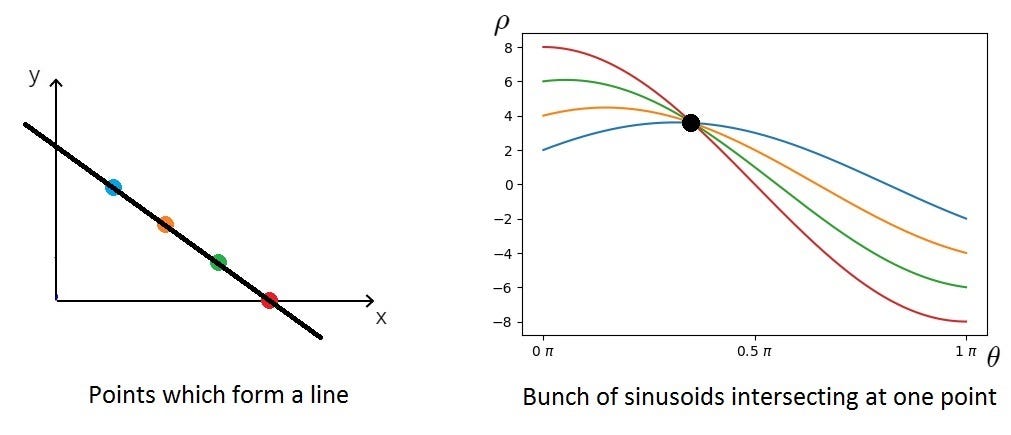
However, the concept remains the same. We’re going to find the bin which has the most intersections and use those m and b values to determine the line of best fit.

So that’s it! I hope you enjoyed that deep dive into the math behind Hough Transform. Now, let’s get back to coding!

Part 3: Optimizing + Displaying the Lines

Now this section about averaging out the lines is made to optimize the algorithm. If we don’t average out the lines, they appear very choppy, since the cv2.HoughLinesP outputs a bunch of mini line segments instead of one big line.

This is without averaging the lines. Pretty choppy, huh.

To average the lines, we’re going to define a function called “average”.

def average(image, lines):
    left = []
    right = []
    for line in lines:
        print(line)
        x1, y1, x2, y2 = line.reshape(4)
        parameters = np.polyfit((x1, x2), (y1, y2), 1)
        slope = parameters[0]
        y_int = parameters[1]
        if slope < 0:
            left.append((slope, y_int))
        else:
            right.append((slope, y_int))

This function averages out the lines made in the cv2.HoughLinesP function. It will find the average slope and y-intercept of the line segments on the left and the right and output two solid lines instead (one on the left and other on the right).

In the output of the cv2.HoughLinesP function, each line segment has 2 coordinates: one denotes the start of the line and the other marks the end of the line. Using these coordinates, we’re going to calculate the slopes and y-intercepts of each line segment.

Then, we’re going to collect all the slopes of the line segments and classify each line segment into either the list corresponding with the left line or the right line (negative slope = left line, positive slope = right line).

• Line 4: Loop through the array of lines
• Line 5: Extract the (x, y) values of the 2 points from each line segment
• Line 6–9: Determine the slope and y-intercept of each line segment.
• Line 10–13: Add the negative slopes to the list for the left lines and the positive slope to the list with the right lines.

NOTE: Normally, a positive slope=left line and a negative slope=right line but in our case, the image’s y-axis is inversed, hence the reason why the slopes are inversed (all images in OpenCV have inversed y-axes).

Next, we have to take the average of the slopes and y-intercepts from both lists.

    right_avg = np.average(right, axis=0)
    left_avg = np.average(left, axis=0)
    left_line = make_points(image, left_avg)
    right_line = make_points(image, right_avg)
    return np.array([left_line, right_line])

Note: Do not place this code inside the for loop.

• Lines 1–2: Takes the average of all the line segments on for both lists (the left side and the right side).
• Lines 3–4: Calculates the start point and endpoint for each line. (We’ll define make_points function in the next section)
• Line 5: Output the 2 coordinates for each line

Now that we have the average slope and y-intercept for both lists, let’s define the start and endpoints for both lists.

def make_points(image, average): 
 slope, y_int = average 
 y1 = image.shape[0]
 y2 = int(y1 * (3/5))
 x1 = int((y1 — y_int) // slope)
 x2 = int((y2 — y_int) // slope)
 return np.array([x1, y1, x2, y2])

This function takes 2 parameters, the image with the lane lines and the list with the average slope and y_int of the line, and outputs the starting and ending points for each line.

• Line 1: Define the function
• Line 2: Get the average slope and y-intercept
• Line 3–4: Define the height of the lines (the same for both left and right)
• Lines 5–6: Calculate x coordinates by rearranging the equation of a line, from y=mx+b to x = (y-b) / m
• Line 7: Output the sets of coordinates

Just to elaborate a bit further, in line 1, we use the y1 value as the height of the image. This is because in OpenCV, the y-axis is inverted, so the 0 is at the top and the height of the image is at the origin (refer to the image below).

Also, in Line 2, we multiplied y1 by 3/5. This is because we want the line to start at the origin ( y1 ) and end 2/5 up the image (it's 2/5 since the y-axis is invested, instead of 3/5 up from 0, we see 2/5 down from the max height).

A visual example of the make_points function applied to the left line

However, this function does not display the lines, it only calculates the points necessary to display these lines. Next, we’re going to create a function which takes these points and makes lines out of them.

def display_lines(image, lines):
 lines_image = np.zeros_like(image)
 if lines is not None:
   for line in lines:
     x1, y1, x2, y2 = line
     cv2.line(lines_image, (x1, y1), (x2, y2), (255, 0, 0), 10)
 return lines_image

This function takes in two parameters: the image which we want to display the lines on and the lane lines which were outputted from the average function.

• Line 2: create a blacked-out image with the same dimensions of our original image
• Line 3: Make sure that the lists with the line points aren’t empty
• Line 4–5: Loop through the lists, and extract the two pairs of (x, y) coordinates
• Line 6: Create the line and paste it onto the blacked-out image
• Line 7: Output the black image with the lines

You may be wondering, why don’t we append the lines onto the real image instead of a black image. Well, the raw image is a little too bright, so it would be nice if we’d darken it a bit to see the lane lines a little more clearly (yes, I know, it's not that big of a deal, but it's always nice to find ways to make the algorithm better)

Left: Appending Lines to Image Directly. Right: Using the cv2.addWeighted function

So all we have to do is call the cv2.addWeighted function.

lanes = cv2.addWeighted(copy, 0.8, black_lines, 1, 1)

This function gives a weight of 0.8 to each pixel in the actual image, making them slightly darker (each pixel is multiplied by 0.8). Likewise, we give a weight of 1 to the blacked-out image with all the lane lines, so all the pixels in that keep the same intensity, making it stand out.

We’re almost at the end of the road (*pun intended). All we have to do is call these functions, so let’s do that right now:

copy = np.copy(image1)
grey = grey(copy)
gaus = gauss(grey)
edges = canny(gaus,50,150)
isolated = region(edges)lines = cv2.HoughLinesP(isolated, 2, np.pi/180, 100, np.array([]), minLineLength=40, maxLineGap=5)
averaged_lines = average(copy, lines)
black_lines = display_lines(copy, averaged_lines)
lanes = cv2.addWeighted(copy, 0.8, black_lines, 1, 1)
cv2.imshow("lanes", lanes)
cv2.waitKey(0)

Here, we simply call all the functions that we previously defined, then we output the result on lines 12. The cv2.waitKey function is used to tell the program how long to display the image for. We passed “0” into the function, meaning it will wait until a key is pressed to close the output window.

Here’s what the output looks like

What the output should look like

We can also apply this same algorithm to a video.

video = r”D:\users\new owner\Desktop\TKS\Article Lane Detection\test2_v2_Trim.mp4"
cap = cv2.VideoCapture(video)
while(cap.isOpened()): 
  ret, frame = cap.read()
  if ret == True:#----THE PREVIOUS ALGORITHM----#
    gaus = gauss(frame)
    edges = cv2.Canny(gaus,50,150)
    isolated = region(edges)
    lines = cv2.HoughLinesP(isolated, 2, np.pi/180, 50, np.array([]), minLineLength=40, maxLineGap=5)
    averaged_lines = average(frame, lines)
    black_lines = display_lines(frame, averaged_lines)
    lanes = cv2.ad1dWeighted(frame, 0.8, black_lines, 1, 1)
    cv2.imshow(“frame”, lanes)
#----THE PREVIOUS ALGORITHM----#
    
    if cv2.waitKey(10) & 0xFF == ord(‘q’): 
      break
  else:
    break
cap.release() 
cv2.destroyAllWindows()

This code applies the algorithm that we created for images into a video. Remember, a video is just a bunch of pictures that appear one after another really quickly.

• Line 1–2: Define the path to the video
• Line 3–4: Capture the video (using cv2.videoCapture ), and loop through all the frames
• Line 5–6: Read the frame, and if there is a frame, continue
• Lines 10–18: Copy the code from the previous algorithm, and replace all the places where we use copy with frame , because we want to make sure we’re operating on the video’s frame not the image from the previous function.
• Lines 22–23: Display each frame for 10 seconds, and if the button “q” is pressed, exit the loop.
• Lines 24–25: Its a continuation of the if statement at lines 5–6, but all its doing is if there isn’t any frame, exit the loop.
• Lines 26–27: Close the video

Alright, you just built an algorithm that can detect lane lines! I hope you enjoyed building this algorithm, but don’t stop here, this is just an intro project into the world of computer vision. Nevertheless, you can brag about building this to your friends :)

Key Takeaways

• Use Gaussian Blur to remove all noise from the image
• Use canny edge detection to isolate edges in the image
• Use Bitwise And function to isolate edges which correspond to the lane lines
• Use Hough Transform to turn the edges into lines

Keywords

If you’re curious, here are the key terms that relate to this algorithm which you can research more in-depth.

• Gaussian Blur
• Bitwise And Binary
• Canny Edge Detection
• Hough Transform
• Gradients
• Polar Coordinates
• OpenCV Lane Line Detection

Other Resources to Consider

• Super well-crafted youtube video. This is where I learned about lane detection, and in fact, my code in this article mostly comes from this video.
• An article by my friend about the same topic.

Next Steps

So where to go after this? There are many things to explore in the world of computer vision. Here are some choices:

• Look into more advanced methods of detecting lines. Hint: Check the Udacity Self-Driving Car Nanodegree Syllabus.
• Look into different computer vision algorithms, here's a great website
• Look into CNN’s, here are my articles on thetheoryand thecode.
• Apply this into a self-driving RC car on Arduino/RasperryPi
• And many more….

That’s A Wrap!

Thanks for reading my article, I really hope you enjoyed it and got some value out of it. I am a 16-year-old computer vision and autonomous vehicles enthusiast who loves building all sorts of machine learning and deep learning projects. If you have any questions, concerns, requests for tutorials, or just want to say hi, you can contact me on Linkedin or Email me.