An introduction to Convolutional Neural Networks

A Convolutional neural network (CNN) is a neural network that has one or more convolutional layers and are used mainly for image processing, classification, segmentation and also for other auto correlated data.

A convolution is essentially sliding a filter over the input. One helpful way to think about convolutions is this quote from Dr Prasad Samarakoon: “A convolution can be thought as “looking at a function’s surroundings to make better/accurate predictions of its outcome.”

Rather than looking at an entire image at once to find certain features it can be more effective to look at smaller portions of the image.

Common uses for CNNs

The most common use for CNNs is image classification, for example identifying satellite images that contain roads or classifying hand written letters and digits. There are other quite mainstream tasks such as image segmentation and signal processing, for which CNNs perform well at.

CNNs have been used for understanding in Natural Language Processing (NLP) and speech recognition, although often for NLP Recurrent Neural Nets (RNNs) are used.

A CNN can also be implemented as a U-Net architecture, which are essentially two almost mirrored CNNs resulting in a CNN whose architecture can be presented in a U shape. U-nets are used where the output needs to be of similar size to the input such as segmentation and image improvement.

Interesting uses for CNNs other than image processing

More and more diverse and interesting uses are being found for CNN architectures. An example of a non-image based application is “The Unreasonable Effectiveness of Convolutional Neural Networks in Population Genetic Inference” by Lex Flagel et al. This is used to perform selective sweeps, finding gene flow, inferring population size changes, inferring rate of recombination.

There are researchers such as Professor Gerald Quon at the Quon-titative biology lab , using CNNs for generative models in single cell genomics for disease identification.

CNNs are also being used in astrophysics to interpret radio telescope data to predict the likely visual image to represent the data.

Deepmind’s WaveNet is a CNN model for generating synthesized voice, used as the basis for Google’s Assistant’s voice synthesizer.

Convolutional kernels

Each convolutional layer contains a series of filters known as convolutional kernels. The filter is a matrix of integers that are used on a subset of the input pixel values, the same size as the kernel. Each pixel is multiplied by the corresponding value in the kernel, then the result is summed up for a single value for simplicity representing a grid cell, like a pixel, in the output channel/feature map.

These are linear transformations, each convolution is a type of affine function.

In computer vision the input is often a 3 channel RGB image. For simplicity, if we take a greyscale image that has one channel (a two dimensional matrix) and a 3×3 convolutional kernel (a two dimensional matrix). The kernel strides over the input matrix of numbers moving horizontally column by column, sliding/scanning over the first rows in the matrix containing the images pixel values. Then the kernel strides down vertically to subsequent rows. Note, the filter may stride over one or several pixels at a time, this is detailed further below.

In other non-vision applications, a one dimensional convolution may slide vertically over an input matrix.

Creating a feature map from a convolutional kernel

Below is a diagram showing the operation of the convolutional kernel.

A stride one 3×3 convolutional kernel acting on a 8×8 input image, outputting an 8×8 filter/channel. Source: https://www.researchgate.net/figure/a-Illustration-of-the-operation-principle-of-the-convolution-kernel-convolutional-layer_fig2_309487032

Below is a visualisation from an excellent presentation, showing the kernel scanning over the values in the input matrix.

Kernel scanning over the values in the input matrix. Source: Otavio Good: excerpt https://www.youtube.com/watch?v=f0t-OCG79-U from https://www.youtube.com/watch?v=Oqm9vsf_hvU

Padding

To handle the edge pixels there are several approaches:

• Losing the edge pixels
• Padding with zero value pixels
• Reflection padding

Reflection padding is by far the best approach, where the number of pixels needed for the convolutional kernel to process the edge pixels are added onto the outside copying the pixels from the edge of the image. For a 3×3 kernel, one pixel needs to be added around the outside, for a 7×7 kernel then three pixels would be reflected around the outside. The pixels added around each side is the dimension, halved and rounded down.

Traditionally in many research papers, the edge pixels are just ignored, which loses a small proportion of the data and this gets increasing worse if there are many deep convolutional layers. For this reason, I could not find existing diagrams to easily convey some of the points here without being misleading and confusing stride 1 convolutions with stride 2 convolutions.

With padding, the output from a input of width w and height h would be width w and height h (the same as the input with a single input channel), assuming the kernel takes a stride of one pixel at a time.

Creating multiple channels/feature maps with multiple kernels

When multiple convolutional kernels are applied within a convolutional layer, many channels/feature maps are created, one from each convolutional kernel. Below is a visualisation below showing the channels/feature maps being created.

Visualisation of channels/feature maps created from a layer of convolutional kernels. Source: Otavio Good: excerpt https://www.youtube.com/watch?v=f0t-OCG79-U from https://www.youtube.com/watch?v=Oqm9vsf_hvU

RGB 3 channel input

Most image processing needs to operate on RGB images with three channels. A RGB image is a three dimensional array of numbers otherwise known as a rank three tensor.

When processing a three channel RGB image, a convolutional kernel that is a three dimensional array/rank 3 tensor of numbers would normally be used. It is very common for the convolutional kernel to be of size 3x3x3 — the convolutional kernel being like a cube.

Usually there is at least three convolutional kernels in order that each can act as a different filter to gain insight from each colour channel.

The convolution kernels as a group make a four dimensional array, otherwise known as a rank four tensor. It is difficult, if not impossible, to visualise dimensions when they are higher than three. In this case imagine it as a list of three dimensional cubes.

The filter moves across the input data in the same way, sliding or taking strides across the rows then moving down the columns and striding across the rows until it reaches the bottom right corner:

3x3x3 convolutional kernel acting on a 3 channel input. Source: https://machinethink.net/images/vggnet-convolutional-neural-network-iphone/[email protected]

With padding and a stride of one, the output from an input of width x, height y and depth 3 would be width x, height y and depth 1, as the cube produces a single summed output value from each stride. For example, with an input of 3x64x64 (say a 64×64 RGB three channel image) then one kernel taking strides of one with padding the edge pixels would output a channel/feature map of 64×64 (one channel).

It is worth noting the input is often normalised, this is detailed further below.

Strides

It is common to use a stride two convolution rather than a stride one convolution, where the convolutional kernel strides over 2 pixels at a time, for example our 3×3 kernel would start at position (1,1), then stride to (1,3), then to 1, 5) and so on, halving the size of the output channel/feature map, compared to the convolutional kernel taking strides of one.

With padding, the output from an input of width w, height h and depth 3 would be the ceiling of width w/2, height h/2 and depth 1, as the kernel outputs a single summed output from each stride.

For example, with an input of 3x64x64 (say a 64×64 RGB three channel image), one kernel taking strides of two with padding the edge pixels, would produce a channel/feature map of 32×32.

Many kernels

In CNN models there are often there are many more than three convolutional kernels, 16 kernels or even 64 kernels in a convolutional layer is common.

These different convolution kernels each act as a different filter creating a channel/feature map representing something different. For example, kernels could be filtering top edges, bottom edges, diagonal lines and so on. In much deeper networks these kernels could be filtering to animal features such as eyes or bird wings.

Having a higher number of convolutional kernels creates a higher number of channels/feature maps and a growing amount of data and this uses more memory. The stride 2 convolution, as per the above example, helps to reduce the memory usage as the output channel of the stride 2 convolution has half the width and height of the input. This assumes reflection padding is being used otherwise it could be slightly smaller.

An example of several convolutional layers of stride 2

With a 64 pixel square input with three channels and 16 3x3x3 kernels our convolutional layer would have:

Input : 64x64x3

Convolutional kernels : 16x3x3x3 (a four dimensional tensor)

Output/activations of the convolutional kernels : 16x32x32 (16 channels/feature maps of 32×32)

The network could then apply batch normalisation to decrease learning time and reduce overfitting, more details below. In addition a non-linear activation function, such as RELU is usually applied to allow the network to approximate better, more details below.

Often there are several layers of stride 2 convolutions, creating an increasing number of channels/feature maps. Taking the example above a layer deeper:

Input : 16x32x32

Convolutional kernels : 64x3x3x3

Output/activations of the convolutional kernels : 64x16x16 (64 channels/feature maps of 16×16)

Then after applying ReLU and batch normalisation (see below), another stride 2 convolution is applied:

Input : 64x16x16

Convolutional kernels : 128x3x3x3

Output/activations of the convolutional kernels : 128x8x8 (128 channels/feature maps of 8×8).

Classification

If, for example, an image belongs to one of 42 categories and the network’s goal is to predict which category the image belongs to.

Following on from the above example with an output of 128x8x8, first the average pool of the rank 3 tensor is taken. The average pool is the mean average of each channel, in the this example each 8×8 matrix is averaged into a single number, with 128 channels/feature maps. This creates 128 numbers, a vector of size 1×128.

The next layer is a matrix or rank 2 tensor of 128×42 weights. The input 1×128 matrix is (dot product) multiplied by the 128×42 matrix producing a 1×42 vector. How activated each of the 42 grid cells/vector elements are, is how much the prediction matches that classification represented by that vector element. Softmax is applied as an activation function and then argmax to select the element highest value.

Rectified Linear Unit (ReLU)

A Rectified Linear Unit is used as a non-linear activation function. A ReLU says if the value is less than zero, round it up to zero.

Normalisation

Normalisation is the process of subtracting the mean and dividing by the standard deviation. It transforms the range of the data to be between -1 and 1 making the data use the same scale, sometimes called Min-Max scaling.

It is common to normalize the input features, standardising the data by removing the mean and scaling to unit variance. It is often important the input features are centred around zero and have variance in the same order.

With some data, such as images the data is scaled so that it’s range is between 0 and 1, most simply dividing the pixel values by 255.

This also allows the training process to find the optimal parameters quicker.

Batch normalisation

Batch normalisation has the benefits of helping to make a network output more stable predictions, reduce overfitting through regularisation and speeds up training by an order of magnitude.

Batch normalisation is the process of carrying normalisation within the scope activation layer of the current batch, subtracting the mean of the batch’s activations and dividing by the standard deviation of the batches activations.

This is necessary as even after normalizing the input as some activations can be higher, which can cause the subsequent layers to act abnormally and makes the network less stable.

As batch normalisation has scaled and shifted the activation outputs, the weights in the next layer will no longer be optimal. Stochastic gradient descent (SGD) would undo the normalisation, as it would minimise the loss function.

To prevent this effect two trainable parameters can be added to each layer to allow SGD to denormalise the output. These parameters are a mean parameter “beta” and a standard deviation parameter “gamma”. Batch normalisation sets these two weights for each activation output to allow the normalisation to be reversed to get the raw input, this avoids affecting the stability of the network by avoiding having to update the other weights.

Why CNNs are so powerful

In simple terms a large enough CNN can solve any solvable problem.

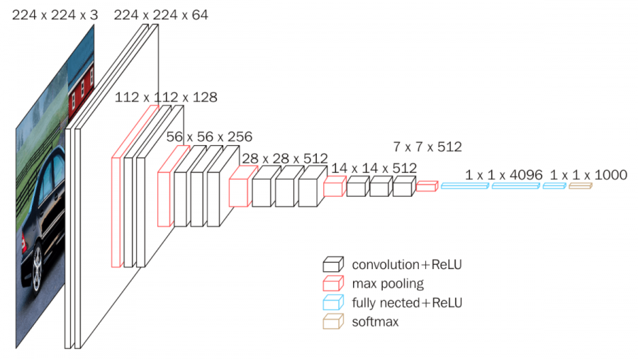
Notable CNN architecture’s that perform exceptionally well across many different image processing tasks are the VGG models ( K. Simonyan and A. Zisserman), the ResNet models (Kaiming He et al) and the Google Inception models (Christian Szegedy et al). These models have millions of trainable parameters.

VGG-16 Network Architecture. Source: https://neurohive.io/wp-content/uploads/2018/11/vgg16-1-e1542731207177.png

Universal approximation theorem

The Universal approximation theorem essentially states if a problem can be solved it can be solved by deep neural networks, given enough layers of affine functions layered with non-linear functions. Essentially a stack of linear functions followed by non-linear functions could solve any problem that is solvable.

Practically in implementation this can be many matrix multiplication with large enough matrices followed by RELU, stacked together these have a mathematical property resulting in being able to solve any arbitrary complex mathematical function to any arbitrary high level of accuracy assuming you have the time and resource to train it.

Whether this would give the neural network understanding is a debated topic, especially by cognitive scientists. The argument is that no matter how well you approximate the syntax and semantics of a problem, you never understand it. This is basically the foundation of Searle’s Chinese Room Argument. Some would argue that does it matter if you can approximate the solution to the problem well enough that it’s indistinguishable from understanding the problem.

Fastai courses

I would like to thank the Fastai team whose courses have helped cement my deep learning and CNN knowledge providing an excellent starting point for further learning and understanding.