E-commerce Analysis: Data-Structures and Applications

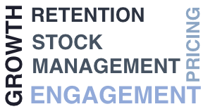
Having effective data structures, enables and empowers different types of analyses to be performed. Overall looking at some of the traditional use cases for e-commerce, we can extract 5 different distinct areas of focus that we might want to address:

We could also add to this data structures related to clickstreams and conversion optimization, marketing spend, product recommendations … but these would need to be the subject of a separate post.

RETENTION STUDIES

Retention studies aim to provide a better understanding which customers stick or depart from the service. They try to find hypotheses as to why customer churn from the platform, hypotheses for which potential treatments can then be tested in live condition.

At the heart of retention studies lies the concept of cohort, typically defined as a group of customer having done their first action at a given point in time. For instance all the customer having made a purchase on your platform on January 2018. We must therefore address cohort modeling as part of the data-structures to be considered.The cohort modeling take as its’ base a table at user level that contains an acquisition date for each customer, for instance:

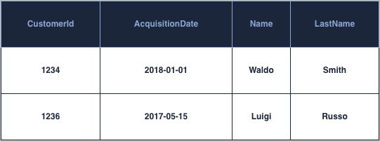
This acquisition date can be based on any activity metrics that you want to consider, be it a sign-up activity, a purchase activity, a website view, … It is

As such this table, lets call it can be populated from any activity table based on an incremental daily load for instance:

As shown above an aggregate event activity is useful for the continuous computation of the dim_customer table.For these metrics it is usually customary to have the event type being tied to the acquistionDate. This enables the nice property that all event activity will be after the acquisition date.

decay histogram

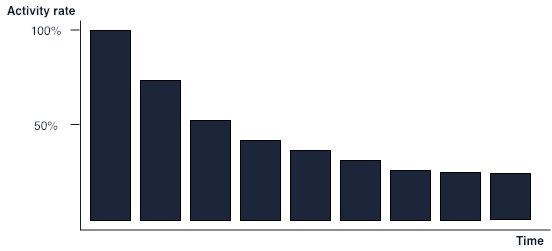
For instance, let’s say that we wanted to compute a decay curve/histogram such as the one depicted on the right. The decay histogram shows the % of a user-base that is active at any given time since acquisition.

Let’s assume that we have built the dim_customer table as shown above based on signup activity and that a signup is the first ever event of a sign-in event.

The above SQL Query for instance enables to compute the datasets needed for this purpose. Since we know that everybody within the user base is active at their Acquisition date (DaySinceAcquisition = 0), we only have to represent D1ActiveCustomers as a proportion of user active at DaySinceAcquisition = 0 to compute the decay histogram.

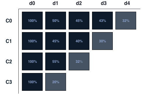
Triangle charts are an evolution of decay curves/histogram, introducing the concept of cohort to the mix. Since we already are computing the acquisition date in order to compute a decay curve, in order to output a triangle chart, the only thing we have to do is to surface that information:

Having other type of attributes within it enables the computation of the datasets needed for repeat purchase rates tables.

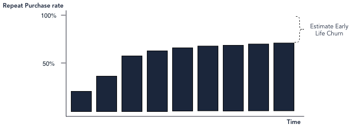
In order to compute the repeat purchase we need to calculate the number of days it took for a given user to achieve his/her second purchase. In this case we still need to keep the concept of cohort in place but we need to augment it with the concept of quantity purchased.

In order to compute the repeat purchase rate, we must first compute for each customer, the number of purchases made with respect to its acquisition date. In a second step we must compute the number of days it took to achieve 2 Purchases. For each customer, we must therefore compute the rollup of all their daily purchases in order to obtain that estimate. Since daily purchases can be numerous (>1), we must further add logic to check that the previous day had less than 2 rolled purchases to identity the date as the repurchase date.

Now let’s assume that we are computing for each day the query: uid_cohort_metrics.sql and providing the result into a table called daily cohort activity. We run the query every day with a filter on activity date that we export as a column:

Based on this table we can compute a daily rollup cohort activity:

After which, we can finally compute effectively the re-purchase rate:

The above query giving us the time and count of customers having turned into a repurchaser after N given days since acquisition. In order to compute the repurchase rate graph, all that is left to do once this dataset is obtained it to make it a running sum and normalize it to the population size.

Setting up a few data-structures based on the above queries significantly helps to get a better understanding how retention behavior across your platform. The most important to setup are a customer level table that contains attributes of the customer both static and computed, customer event aggregation tables and customer cohort level tables. Having these setup makes it fairly easy to retrieve the information necessary in order to compute the different retention graphs and charts, from decay curves, triangle charts to repeat purchase histograms.

ENGAGEMENT STUDIES

Different framework for understanding customer engagement exists out there. They exist to understand how different segment of the customer base interact with your platform. Two of the most frequent frameworks used to get a sense of engagement are RFM and power user curves.

RFM is a segmentation methodology that works through the computation of 3 specific dimension, recency, frequency and monetary value. The RFM then place a score for each customer across each of these dimensions, with the higher values representing the most desirable outcome.

The first dimension, recency can be obtained by a slight modification to the dim_purchaser table and query to include a last purchase date.

The frequency and monetary value metrics are normally taken as being trailing metrics such as trailing measurements such as trailing twelve months ( TTM ). These calculation can be made by enhancing the daily rollup cohort activity query with a value measure and the necessary trailing metrics.

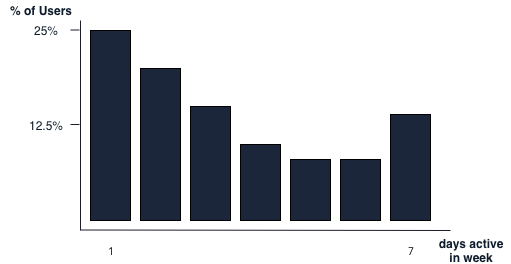
Power User curves are a different mean to get some information as to how your customer base is trending in terms of activity. It relies on a metrics of days of activity, Facebook had defined an L30 measure to define the total number of days, users were active in a given month. The shape and trend of the power user curves gives a sense of user activity and engagement within the time period, allowing the identification of power users across the customer base. An L28 measure is sometimes used instead of an L30 measure as a proxy for the monthly activity, due to the computational advantages of L28. L28 can be computed as the sum of four L7 weekly measures, and l7 measures themselves can be computed as the sum of 7 L1.

Engagement studies only need little tweaks on the data-structures needed for retention studies in order to be catered for. At their core, they rely on information being available at customer level with trailing measures, and these measures be grafted on those needed for retention studies with ease.

GROWTH ACCOUNTING

Growth Accounting attempts to split your customer base into different lifestage status and understand the evolution of your active customer base through these statuses. For this purpose A customer can be in a stage of a new customer, a resurrected, retained, churned or potentially stale.

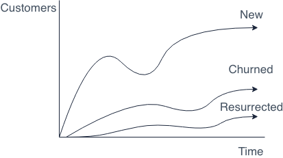
Growth Accounting can help you understand if you are effectively retaining or resurrecting your customer for effective growth or if you are facing a headwind with respect to growth due to churn.

The definition of Active User/Customers within growth accounting is primordial, it usually refers to users having performed a given action in the past X days.

The following two equations define how growth accounting is split out across lifestage:

Active(t) = New(t) + Resurrected(t) + Retained(t)

Retained(t) = Active(t-1) — Churned(t)

For a more thorough explanation of growth accounting:

In essence growth accounting assign to a user a status based on its’ activity today and his activity status of yesterday. Let’s say we have two tables, one containing the daily Lx values for customers the other meant to store the growth accounting status of the customers, then we could compute the new growth accounting status like this:

The status column for growth accounting could be potentially added to any date / customer table already existing to provide that information. For instance if dim_customers contained a snapshot of all customers present on a given date the growth accounting status could potentially be placed there.

PRICING STUDIES

There is a wide range of pricing studies that are of interest on a website, from study of change in Price Discount Perception (Sales Price / Recommended Retail Price), Price Elasticities, revenue cannibalization …

For pricing studies it is important to have a snapshot table or a type II history table that contains the pricing history of each item available on the website.

A snapshot table would contain the state of the different prices active on a given day / hour etc.. If price would change within that interval only one of the value would be captured. Nevertheless the use of a snapshot table in order to study pricing behavior can be quite effective. It allows for simple query to be run and see how price has impacted purchasing behavior for instance.

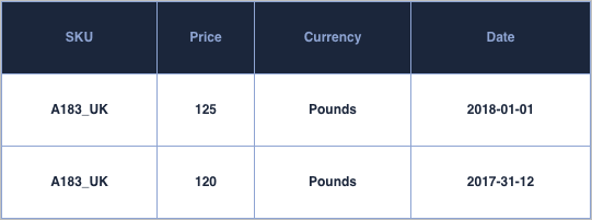
Depending on the source system used, it might be difficult to understand when a price has been change and have a certain history or pricing changes. In these cases a snapshot table is recommended, where the data feeding into it would be obtained at certain recurring intervals. Simple queries can be run on these type of tables to understand for instance when prices have been changed:

As well as for instance getting a quick understanding of the discount level active on the site:

Price snapshots tables makes these kind of queries fairly easy to compute.

Another data structure that is useful for pricing studies is history or type II tables. Type II tables hold pricing information that is valid for a certain range of time as shown in the table below:

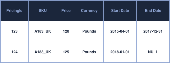
Since type II table holds a range, they can handle without any issues granular switchover, for instance they could host a start_time in milliseconds to provide the information as to how long the given price was active. Beside this, the main advantage of this data structure compared to a price snapshot is the significantly lower size of the table when price changes occurs at a low-medium frequency.

Type II history table can for instance be particularly useful for pricing studies to understand how much we should per day based on each pricing period:

Overall both snapshot and history tables help shed lights to diverse pricing studies. Having both data structures helps gain efficiencies in the analysis of pricing movements but it is however necessary to take into account the limitations of snapshot tables within these analyses.

Stock Management

Efficient inventory management can sometimes be challenging depending on the data-feed that are provided. The minimum that is needed to be able to run a web-shop only relies on two columns SKU and quantity sellable. For analytics purposes a lot more attributes is desirable.

For instance to deal with perishable products, both having visibility of lot number and expiration date would allow for visibility on the products likely to be scrapped. For goods receipt and damaged goods having a status within inventory would allow to better understand what volume of the SKU could potentially be repaired/refurbished and put back into inventory or salvaged for spare parts.

One potential use of this data-structure is to calculate the number of days on hand (doh) of inventory. Days on Hand is a measure to understand if we might be over or understocked for particular items. If for instance we wanted to calculate doh based on the trailing 7 days sales using this data structure:

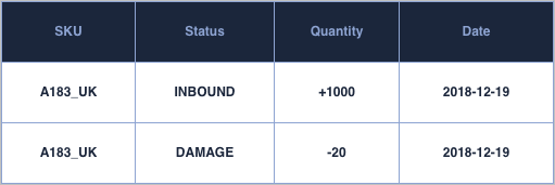
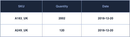
Inventory variation is another topic in stock management, that requires its own data structures. Having visibility on the cause of inventory movement helps shed light on what happens operationally, be it damages, inventory transfers across warehouses or stock inbound. At the very minimum a data-structure should contain SKU information, status code, quantity and date of the movements:

Having this information can allow us for instance to both reconcile our stock position as the sum of these events, but also for instance to calculate KPIs such as damage rate as well as other operational metrics.

Wrapping up

Retention, Engagement and Growth are all user focused area and it is therefore no surprise that they would require similar data-structures to be built to cater for their analysis and reporting, namely:

• customer table
• customer event aggregate
• customer cohort aggregates.

Pricing studies can in turn rely on two type of data structure to help with the analysis, essentially containing the same information, but making certain queries on it more accessible, Price Snapshots and Price History tables.

Stock management in turn also relies on two data structure an Inventory table and an inventory variation table. The inventory table is highly dependent on the number of attributes and granularity that can be obtained from source systems, while inventory variation table might be construed as a consolidation of multiple events.

E-Commerce is a vast domain that enables a wide scope of analysis and having efficient data structure such as those listed above that helps with that provide significant value.